Sloshing Suppression Control by using Physical Boundary Element
Model and Predictive Control in Liquid Container Transfer System
Hisashi Okatsuka
1
, Ryota Shibuya
1
, Kazuhiko Terashima
1
, Yoshiyuki Noda
2
and Yoshiki Matsuo
3
1
Department of Mechanical Engineering, Toyohashi University of Technology,
Hibarigaoka 1-1, Tempaku, Toyohashi, Aichi 441-8580, Japan
2
Department of Mechanical System Engineering, Faculty of Engineering, University of Yamanashi,
Takeda 4-4-37, Kofu, Yamanashi 440-0016, Japan
3
Department of Computer Siecnce, Tokyo University of Technology,
1404-1 Katakuramachi, Hachioji City, Tokyo 192-0982, Japan
Keywords:
Sloshing Control, Boundary Element Method, Generalized Predictive Control.
Abstract:
This paper presents sloshing suppression control of liquid transferred at a desirable-speed. In order to suppress
sloshing, a mathematical model consisting of continuous equations and the pressure equation is used and the
sloshing phenomena are analyzed by using the Boundary Element Method (BEM). Further, the BEM model is
transformed into the state-variable model. The proposed model can estimate not only first-order mode sloshing
but also higher-order mode sloshing and predict the future behavior of liquid level more precisely. Moreover,
sloshing is suppressed by using Model Predictive Control (MPC). We were able to transfer the container while
minimizing sloshing and maintaining a desirable speed.
1 INTRODUCTION
In recent years, multi-kind and small-quantity pro-
duction has become mainstream in manufacturing in-
dustry to meet customer needs. However, increas-
ing complexity of manufacturing lines and the ris-
ing number of processes have resulted in higher man-
ufacturing costs and the need for frequent mainte-
nance. Furthermore, types of liquid products range
from food to chemicals and molten metals. Piping
systems are generally used for tranferring these liq-
uid products. High-pressure water techniques using
pumps are widely applied for washing these piping
systems. However, the need for frequent washing and
maintenance has led to cost increases and deteriora-
tion of production efficiency. Therefore, there is a
need for a reasonable liquid transfer system with ease
of maintenance and a simple mechanism.
In this paper, we propose a transfer system for
liquid containers, which is combined with a servo
motor. The proposed system is easy to maintain.
However, during high-speed transfer of containers,
sloshing (liquid vibration) occurs on the liquid surface
and may causes liquid overflow and/or quality deteri-
oration owing to entrainment of air or gases. There-
fore, a newapproach is required to enable transferring
Figure 1: Photos of experimental results.
liquid containers at a desirable speed while suppress-
ing sloshing.
Fig. 1 shows the motion of the liquid surface. The
left photo shows the case without control and the right
photo shows the case with control. These are images
captured when the container was stopped after being
transferred for 0.3 m.
Concerning sloshing analysis, computer simula-
tion and anti-slosh structure design, much research
has been reported since the 1960s(Abramson and
Chu, 1966)(Ibrahim, 2005). On the other hand, dy-
namic control of sloshing has been studied since
1990. Major studies on sloshing control include one
using a simple pendulum and an optimal servo sys-
tem combined with a kalman filter (Hamaguchi et al.,
1994). Yano, Oguro and Terashima (Yano et al.,
2001) omitted the frequency area of the input sig-
nal around the peak of the transfer function in or-
507
Okatsuka H., Shibuya R., Terashima K., Noda Y. and Matsuo Y..
Sloshing Suppression Control by using Physical Boundary Element Model and Predictive Control in Liquid Container Transfer System.
DOI: 10.5220/0004037705070512
In Proceedings of the 9th International Conference on Informatics in Control, Automation and Robotics (ICINCO-2012), pages 507-512
ISBN: 978-989-8565-22-8
Copyright
c
 2012 SCITEPRESS (Science and Technology Publications, Lda.)

der to eliminate vibration. Furthermore, Romero
et al.referred to many reports concerning numerical
analysis of liquid in rectangular containers subjected
to horizontal acceleration (Romero and Ingber, 1995).
Feddema et al. (Feddema et al., 1997) proposed meth-
ods for controlling the surface of a liquid in an open
container by altering the horizontal acceleration or by
tilting the container parallel with the liquid surface
in order to suppress sloshing. Mathematical models
that have been proposed are mostly for the first-order
mode sloshing in order to suppress vibration on the
walls of containers. However, in a container tran-
ferred at a reasonable speed, higher-order model of
vibration is caused, and it is impossible to estimate
sloshing accurately by using the conventional model.
Other research applies the Boundary Element
Method (BEM)(Nakayama and Washizu, 1981) to di-
vide the liquid surface into multiple boundary points
and calcurate the surface displacement at each point.
For this analysis, the continuous formula of the liquid
and the boundary condition of the surface are neces-
sary. When this approach is applied to sloshing con-
trol, the modal model with a suitable degree is built,
where model parameters are identified by the curve
fitting method, comparing with the results of BEM
simulations (Hamaguchi et al., 1995). This proce-
dure causes the mathematical model based on BEM
to lose its physical structure and be transformed into
a black-box model. Therefore, in this paper, a BEM
model(Okatsuka et al., 2002) is translated to a state
space model based on physical differential equations
expressing the liquid surface displacement.
Figure 2: Analytical model of liquid container.
This linear system clarifies the relations between
inputs and outputs, including the higher-mode vibra-
tion, and enables reasonable control of sloshing, when
combined with modern control theory. The optimum
control of sloshing is achieved by the combination
with model predictive control (MPC). With regard to
MPC, generalized predictive control (GPC)(Oshima,
2000)(Masuda et al., 2000) is used in this paper.
2 BASIC EQUATIONS AND
ANALYSIS CONDITIONS
In this section, we explain the governing equa-
tions(Kimura et al., 1996), analysis conditions and the
target container.
• Ω is the area occupied with liquid. The boundary
Γ is composed of two boundaries, Γ
f
and Γ
w
. Γ
f
is the free surface in contact with the air and Γ
w
is
the wall surface. Thus, Γ = Γ
f
+ Γ
w
.
• The number of elements by BEM : Total of 60 ele-
ments comprising 20 elements on the free surface
and on the bottom, respectively, and 10 elements
on the side wall. Elements are counted counter-
clockwise at the boundry.
• The liquid is a perfect fluid that has no vortex or
viscosity, and is incompressible. The pressure on
the free surface is constant, and the displacement
is assumed to be minute.
• The center of moving and pitching vibration
C(x
c
,0,z
c
) is on the z-axis (x
c
= 0).
• The velocity potential Φ(x,z,t) is defined by the
relative velocity of the liquid corresponding to the
container.
• The control value (output), the displacement from
the liquid surface at rest η(x,t)[m], is the motion
relative to the container.
• The manipulator forces are the displacement ac-
celeration
¨
f
X
(t) [m/s
2
] in the X direction and
the angular acceleration of pitching excitation
¨
ξ(t)[rad/s
2
]. These forces are moved by a ma-
nipulator through the control signal. The forced
displacement in the Z-direction f
z
(t)[m] = 0.
∂
2
Φ
∂x
2
+
∂
2
Φ
∂z
2
= 0 (1)
∂Φ
∂x




x=±a
= 0
∂Φ
∂z




z=0
= 0 ; on Γ
w
(2)
∂Φ
∂t




z=h+η
+ x[
¨
f
X
− g∗ ξ]
+x[(h− z
c
)
¨
ξ] + g ∗ (η + h+ f
Z
) = 0 (3)
∂Φ
∂t




z=h+η
=
∂η
∂t
− 2x
˙
ξ ; on Γ
f
(4)
(1. Laplace equation; expressing the condition of
continuity inside the liquid
(2. Adaptable condition on the side wall and the base
(3. Dynamic boundary condition on the liquid surface
(4. Kinematic boundary condition on the liquid sur-
face
In the above-mentioned basic equations, non-
linear parts are eliminated. Hhereafter, f
z
= 0 in all
equations.
ICINCO2012-9thInternationalConferenceonInformaticsinControl,AutomationandRobotics
508

3 DERIVATION OF THE
BOUNDARY INTEGRAL
EQUATION
Assuming ζ and x(x,z) as the random point on the
boundary, the boundary problem of two dimensions is
solved using the weighted residual expression. Here,
α is the internal angle at the point ζ.
α(ζ)
2π
Φ(ζ,t) +
Z
Γ
Φ(x,t)q
∗
(x,ζ)dΓ(x)
−
Z
Γ
∂Φ
∂n
v
∗
(x,ζ)dΓ(x) = 0 (5)
Here, the following formulas are employed as the ba-
sic solutions. Here,B!H(BnB!I(Bshows the outward
normal at the boundary.
q
∗
(x,ζ) =
1
2π
∂
∂n
(ln
1
r
), v
∗
(x,ζ) =
1
2π
(ln
1
r
),
where r = k x − ζk. Substitute the boundary con-
ditions Eq. 2 and Eq. 4 into the Eq. 5 ,where
∂Φ/∂n = ∂Φ/∂z, and the following equation is ob-
tained:
α(ζ)
2π
Φ(ζ,t) +
Z
Γ
f
+Γ
w
Φ(x,t)q
∗
(x,ζ)dΓ(x)
−
Z
Γ
f
[
˙
η(x,t) − 2x
˙
ξ]v
∗
(x,ζ)dΓ(x) = 0
In order to solve the above equation using
the boundary collocation method
1
,suppose x
i
(i =
1,2,··· ,N) as the coordinates of the collocation.
Then, the following equation is obtained :
α(x
i
)
2π
Φ(x
i
,t) +
Z
Γ
f
+Γ
w
Φ(x,t)q
∗
(x,x
i
)dΓ(x)
−
Z
Γ
f
[
˙
η(x,t)s− 2x
˙
ξ]v
∗
(x,x
i
)dΓ(x) = 0 (6)
Concerning Eq. 3, which represents the dynam-
ical boundary condition, we suppose that the first
M pieces x
j
( j = 1,2,··· ,M) of collocation (in all
pieces) exist on the free surface Γ
f
.
˙
Φ(x
j
,t) + x
j
[
¨
f
X
− g∗ ξ]
+x
j
[(h− z
c
)
¨
ξ] + g(η(x
j
,t) + h) = 0 (7)
By these procedures, the basic equations (Eq.1 ∼
Eq.4) are transformedto simultaneous equations com-
prising an integral equation (6) and a boundary con-
dition (7).
1
The Boundary collocation method selects limited
points on the boundary and makes the residual zero.
4 DISCRETE-TIME SYSTEM AND
STATE EQUATIONS
In order to organize a discrete-time system, the
boundary Γ is divided into many straight-line ele-
ments, and Eq. 6 becomes as follows. However, the
values of Φ and η in each element are fixed.
α(x
i
)
2π
Φ(x
i
,t) +
∑
Γ
f
+Γ
w

Z
e
j
Φ(x,t)q
∗
(x,x
i
)dΓ(x)

−
∑
Γ
f

Z
e
j
[
˙
η(x,t) − 2x
˙
ξ]v
∗
(x,x
i
)dΓ(x)

= 0 (8)
where Φ(x,t) = Φ(x
j
,t) = Φ
j
,
˙
η(x,t) =
˙
η(x
j
,t) =
˙
η
j
and α(x
i
) = π
1
2
Φ(x
i
,t) +
∑
Γ
f
+Γ
w

Z
e
j
q
∗
(x,x
i
)dΓ(x)

Φ
j
−
∑
Γ
f

Z
e
j
v
∗
(x,x
i
)dΓ(x)

˙
η
j
+2
∑
Γ
f

Z
e
j
v
∗
(x,x
i
)dΓ(x)

x
j
˙
ξ = 0 (9)
Furthermore, using the influence parameters
ˆ
H
ij
and G
ij
, defined by the following formulas, Eq. 9
becomes Eq. 10.
ˆ
H
ij
≡
Z
e
j
q
∗
(x, x
i
)dΓ(x)
=
1
2π
Z
e
j
∂
∂n(x)

ln
1
kx− x
i
k

dΓ(x)
(i = 1 ∼ 60, j = 1 ∼ 60)
G
ij
≡
Z
e
j
v
∗
(x, x
i
)dΓ(x)
=
1
2π
Z
e
j

ln
1
kx− x
i
k

dΓ(x)
(i = 1 ∼ 60, j = 1 ∼ 20)
1
2
Φ(x
i
,t) +
∑
Γ
f
+Γ
w
ˆ
H
ij
Φ
j
=
∑
Γ
f
G
ij
˙
η
j
− 2
∑
Γ
f
G
ij
x
j
˙
ξ
(10)
Next, in order to arrange the left side for Φ
j
, substitute
ˆ
H
ij
by H
ij
(here,
ˆ
H
ij
= 0 for i=j),
2
and the following
is obtained :
H
ij
≡
1
2
δ
ij
+
ˆ
H
ij
=
ˆ
H
ij
(i 6= j)(δ
ij
= 0)
H
ij
≡
1
2
δ
ij
+
ˆ
H
ij
=
1
2
(i = j)(δ
ij
= 1)
2
When the collocation is consistent with the node, the
normal vector at point X intersect orthogonally with the
vector (X − X
i
)
SloshingSuppressionControlbyusingPhysicalBoundaryElementModelandPredictiveControlinLiquidContainer
TransferSystem
509

The output equation is as follows :
M
∑
j=1
G
ij
˙
η
j
=
N
∑
j=1
H
ij
Φ
j
+ 2
M
∑
j=1
G
ij
x
j
˙
ξ
(N > M, i = 1,2,··· ,N) (11)
Furthermore, divide Eq. 11, top and bottom, right
and left, in order to eliminate Φ that is larger than M.



˙
η
1
.
.
.
˙
η
M



=

P
−1
Q




Φ
1
.
.
.
Φ
M



+ 2



x
1
.
.
.
x
M



˙
ξ,
(12)
where
P = (G
1
) − (H
2
)(H
4
)
−1
(G
2
)
Q = (H
1
) − (H
2
)(H
4
)
−1
(H
3
) (13)
G
1
= G
ij
(1 ≤ i ≤ M, 1 ≤ j ≤ M)
H
1
= H
ij
(1 ≤ i ≤ M, 1 ≤ j ≤ M)
H
2
,G
2
,H
3
,H
4
are similar to above. Next, in the dy-
namic boundary Eq. 7 for the free liquid surface,
leave the differential item on the left side of the equal
sign:



˙
Φ
1
.
.
.
˙
Φ
M



= −g



η
1
.
.
.
η
M



+ [(z
c
− h)x
j
¨
ξ] + gx
j
ξ
−(
¨
f
X
x
j
+ gh)
( j = 1,2, · · · ,M) (14)
Exciting angular acceleration and exciting angular ve-
locity are as follows :
(
˙
˙
ξ) =
¨
ξ,
˙
(ξ) =
˙
ξ
Consequently, the state equation using a state variable
vector of X = (Φ
1···M
,η
1···M
,
˙
ξ,ξ)
T
becomes
˙
X = AX+ b


(
¨
ξ)
¨
f
X
h


, (15)
where
A =



0
M
−gI
M
0 gx
j
(P
−1
Q) 0
M
2x
j
0
0 0 0 0
0 0 1 0



,
b =














(z
c
− h)x
j
−x
j
−g
.
.
.
−g





M
0
.
.
.
0
0
.
.
.
0
0
.
.
.
0





M
1 0 0
0 0 0














The output equation is as follows :
z =

η
1
,η
2
,··· ,η
M

= cX, (16)
where
c =

0
1···M
, 1
1···M
, 0, 0

Furthermore, using MATLAB, [A
G
,b
G
] =
c2d(A,b,τ), consider k as the parameter for the
sampling period τ (=0.01[s]), and the following
equation is obtained :
˙
X[k+ 1] = A
G
X[k] + b
G


(
¨
ξ[k])
¨
f
X
[k]
h


(17)
The right side of the Eq. 17,
¨
ξ[k] and
¨
f
X
[k], is the
control input.
5 EXPERIMENTAL APPARATUS
AND VERIFICATION OF THE
MODEL
The external appearance of the experimental appara-
tus is shown in Fig. 3. The container made of acrylic
resin, which is attached to the end point of the arm
supported by the z-axis, is moved by the AC serve
motor along the Y-axis ( 0.3[m] in distance), while
rotating around the T-axis. The slender bar vertically
mounted on the right side of the container is a level
sensor for measuring the behavior of the liquid sur-
face. This sensor is composed of two pieces of stain-
less wire with a diameter of 3×10
−3
[m] placed in par-
allel with an intervalof 0.01[m], which are electrodes.
Using this apparatus, the values of the simulation and
the experimental data are compared.
Figure 3: Experimental equipment.
Fig. 4(a), (b) and (c) show transferring position,
velocity and acceleration, respectively. Fig. 4(d)
shows the estimate and the experimental data for the
liquid surface vibration. They are in good agreement.
ICINCO2012-9thInternationalConferenceonInformaticsinControl,AutomationandRobotics
510

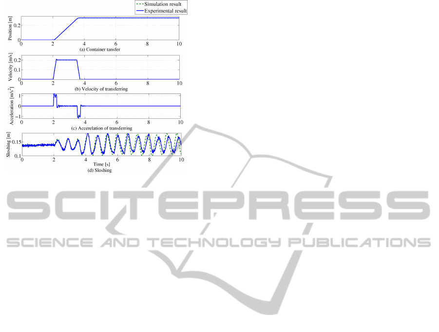
Figure 4: Experimental results for transferring a container.
6 DERIVATION OF THE
OPTIMAL CONTROL INPUT
AND EXPERIMENTAL
RESULTS
The state variables X obtained in the previous section
and Eq. 16 and Eq. 17 are shown again. We are able
to develop the optimal control law from these items,
which constitute a plant model. Since the target value
is not step-formed, a special formula including an in-
tegrator is not employed. Moreover,instead of the in-
crement of the input, the input itself is used.
X = (Φ
1···M
, η
1···M
,
˙
ξ, ξ)
T
X[k+ 1] = A
G
X[k] + b
G
(
¨
ξ[k])
¨
f
X
[k]
h
!
z[k] = cX[k]
Assuming that the value of the angular acceleration
¨
ξ
of the container is zero, the above formulas are used
again to eliminate the constant terms, and a predictive
formula for the output is obtained as follows. Here,
b
G
= [b
G1
,b
G2
,b
G3
]
ˆ
z[k+ j] = cA
G
j
X[k] +
j−1
∑
i=0
cA
G
j−i−1
(b
G2
¨
f
X
[k+ i])
(18)
The first term of the right side depends on the state
at time [k] and the second term depends on the fu-
ture control input (on condition that 0 ≤ i ≤ j − 1).
Next, in order to use GPC theory, the following linear
quadratic evaluation function is given. Q and R are
the weighted matrix for the liquid surface variation
and control input.
J =
N
2
∑
j=N
1
ˆ
z[k+ j]
T
Q
ˆ
z[k+ j]
+
N
u
∑
j=1
¨
f
X
[k+ j − 1]
T
R
¨
f
X
[k+ j − 1](19)
The above formula is obtained from two conditions.
Firstly, the future target for the output is zero. Sec-
ondly,
¨
f
X
is applied for the input. N
1
and N
2
are the
minimum and maximum prediction area, respectively,
and N
u
is the control prediction area. We adopted
N
1
= 1, N
2
= 4 and N
u
= 3. We used as small values as
possible for N
1
, N
2
and N
u
in order to increase the cal-
culation speed of the experimental apparatus. As the
results obtained by using these values were desirable,
we employed these values. Furthermore, concerning
Q and R, considers to become on the same level of
size. The predictive formula for output is expressed
in the vector form as follows in order to obtain the
optimum control law.
J = (Z[k])
T
Q(Z[k]) + D[k]
T
RD[k], (20)
where
Z[k]
T
= [
ˆ
z[k+ N
1
]
T
,··· ,
ˆ
z[k+ N
2
]
T
]
D[k]
T
= [
¨
f
X
[k]
T
,··· ,
¨
f
X
[k+ N
u
− 1]
T
]
Z[k] = G
s
D[k] + H
s
X[k] (21)
G
s
=




cb
G1
0 0
cA
G
b
G1
cb
G1
0
cA
2
G
b
G1
cA
G
b
G1
cb
G1
cA
3
G
b
G1
cA
2
G
b
G1
cA
G
b
G1




,
H
s
=

cA
G
, cA
2
G
, cA
3
G
, cA
4
G

T
Substitute Eq. 21 into Eq. 20, and the control
inputD[k] that minimizes the value of the evaluation
function becomes as follows :
D[k] = (G
T
s
QG
s
+ R)
−1
Gs
T
Q(−H
s
x[k]) (22)
The above control law is effective between time[k]
and time[k + N
u
− 1]. However, as mentioned above,
the influence of the state of the control object and
the disturbance at the current time only are taken into
consideration. Therefore, the control law gives the in-
put at the current time only. Thus, the first block of
D[k] is applied to the control object as follows-:
¨
f
X
[k] = [I
m
,0,··· ,0] D[k] (23)
Fig. 5 shows the control result using GPC. This
figure shows good sloshing suppression. In order
to evaluate the effectiveness of the proposed con-
trol method, the proposed method and a conventional
method using a notch filter are compared. The notch
filter eliminates the input gain based on the sloshing
natural frequency (Yano and Terashima, 2001). Fig.
6 shows the experimental results.
SloshingSuppressionControlbyusingPhysicalBoundaryElementModelandPredictiveControlinLiquidContainer
TransferSystem
511

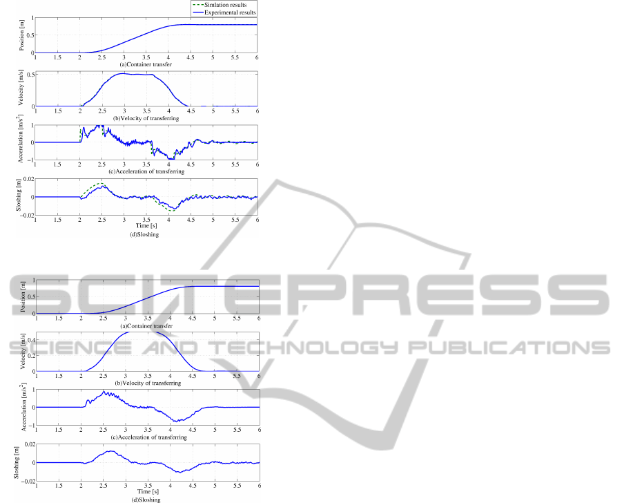
Figure 5: Experimental results (GPC control case).
Figure 6: Experimental results (use of a notch filter).
7 CONCLUSIONS
Using the state-space equation obtained using BEM,
we were able to precisely express the liquid surface
vibration during transfer and tilting of a container.
Moreover, using GPC, we were able to keep the liquid
surface flat during transfer of the container at a con-
stant speed when acceleration is applied in the hori-
zontal direction. In particular, we achieved immedi-
ate suppression of sloshing when the container stops.
Experimental results provide evidence that our con-
trol approach using both the BEM model and MPC
achieves better results than any conventional control
methods such as the notch filter technique and PID
control. Furthermore, useful research based on this
paper was reported (Shibuya et al., 2011)
REFERENCES
Abramson, H. and Chu, W.H.and Kana, D. (1966). Some
studies of non-linear lateral sloshing in rigid contain-
ers. J.Appl. Mechanics, Trans. ASME, 1966, pages
777–784.
Feddema, J., Dohrmann, C., Parker, G., Robinett, R.,
Romero, V., and Schmitt, D. (1997). Control for slosh-
free motion of an open container. IEEE Trans. on Con-
trol Systems Technology, 5(1):29–36.
Hamaguchi, M., Motegi, H., Terashima, K., and Nomura,
N. (1995). Optimal control of transferring a liq-
uid container with boundary element analysis, (in
japanese). Trans. of the Society of Instrument and
Control Engineers (SICE), 31(9):1442–1451.
Hamaguchi, M., Terashima, K., and Nomura, H. (1994).
Optimal control of transferring a liquid container
for several performance specifications, (in japanese).
Trans. of the Japan Society of Mechanical Engineers
(JSME) C, 60(573):1668–1675.
Ibrahim, R. (2005). Liquid Sloshing Dynamics. Cambridge
Univ.
Kimura, K., Takahara, H., and Sakata, M. (1996). Sloshing
in a circular cylindrical tank subjected to pitching ex-
citation (condition for liquid surface remaining plane).
Trans. of the Japan Society of Mechanical Engineers
(JSME), (96-1):1321.
Masuda, S., Shah, S., and Gopaluni, R. (2000). An adap-
tive state-space based gpc with a two-degrees-of free-
dom controller structure. In IFAC Advanced Control
of Chemical Processes.
Nakayama, T. and Washizu, K. (1981). The bound-
ary element method applied to the analysis of two-
dimensional nonlinear sloshing problems. Int. J. for
Numerical Methods in Engineering, 17:1631–1646.
Okatsuka, H., Matsuo, Y., and Inaba, T. (2002). Sloshing-
less manipulation of liquid in open-type containers,
(in japanese). Trans. of Simulation Technology Con-
ference, pages 161–164.
Oshima, M. (2000). Model predictive control (in japanese).
Trans. of the Society of Instrument and Control Engi-
neers (SICE), 39(5):321–325.
Romero, V. and Ingber, M. (1995). A numerical model
for 2-d sloshing of pseudoviscous liquids in horizon-
tally accelerated rectangular containers. Boundary El-
ements XVII, pages 567–583.
Shibuya, R., Okatsuka, H., Noda, Y., and Terashima, K.
(2011). Transferring and tilt motion control of the
liquid container to suprerss slothing by using gpc.
In IEEE/SICE International Symposium, pages 1055–
1060.
Yano, K., Oguro, N., and Terashima, K. (2001). Starting
control with vibration damping by hybrid shaped ap-
proach considering time and frequency specifications,
(in japanese). Trans. of the Society of Instrument and
Control Engineers (SICE), 37(5):403–410.
Yano, K. and Terashima, K. (2001). Robust liquid con-
tainer transfer control for complete sloshing suppres-
sion. IEEE Trans. on Control Systems Technology,
9(3):483–493.
ICINCO2012-9thInternationalConferenceonInformaticsinControl,AutomationandRobotics
512