
State Estimation and Send on Delta Strategy Codesign for Networked
Control Systems
∗
Ignacio Pe˜narrocha, Daniel Dolz, Julio A. Romero and Roberto Sanchis
Dep. Enginyeria de Sistemes Industrials i Disseny, University Jaume I, Campus de Riu Sec, Castell´on, Spain
Keywords:
State Estimation, Networked Control, Send on Delta, Event based Estimation and Control.
Abstract:
In this work, a new strategy to minimize the use of the network in state estimation over networks is addressed,
leading to a co-design procedure of both the observer and the policy for message sending. The sensor nodes
implements a send-on-delta approach, sending new data only when there is a considerable deviation from the
last sent measurement. The estimator node implements a gain scheduling approach that takes into account
the availability of new received data. The performance of the observer is analyzed through H
∞
norm in both
deterministic and stochastic data transfer rate. This norm is used to design both the observer gains and the
output variations that induce the sensors to send new outputs to the estimator node, while guaranteeing a given
level of performance on the state estimation error. The design approach is based on an optimization procedure
with linear and bilinear matrix inequalities constraints that is solved iteratively.
1 INTRODUCTION
The reduction of data traffic through the communica-
tion networks while obtaining acceptable closed loop
performance, is the main goal in many networked
control systems design methodologies. Co-design
strategies, where communication can be optimized
with respect to the controller’s stability and/or perfor-
mance, represent in the last years a widely accepted
approach to deal with this problem, (Wang and Lem-
mon, 2009; Dai et al., 2010; Gaid et al., 2006; Irwin
et al., 2010).
State estimation play a key role in networked con-
trol systems, because in most of the practical appli-
cations the full state of the plant is not available for
control purposes. Many algorithms have been pro-
posed considering remote sensor nodes that send data
over the network to an estimation node. Co-design
has also been extended, taking into account both the
estimation quality and the communication issues, to
the solution of this problem: optimize the network us-
age while guaranteing a given estimation requirement
such as a prescribed state estimation error covariance.
(Marck and Sijs, 2010) proposes the design of a mea-
surement sampling protocol that is used in combina-
tion with an event-based state-estimator. The protocol
minimizes communication resources and the state es-
∗
This work has been supported by MICINN project
number DPI2011-27845-C02-02.
timation is accurate and remains stable even when no
samples are sent.
In this paper a new methodology for estimator
co-design is presented, which considers the send-on-
delta (SOD) transmission between the sensor nodes
and the estimator node. The SOD method consists
of transmitting data from the sensor to the estima-
tor node only if the measurement value changes more
than a given specified ∆ value, (Miskowicz, 2006).
Previous works on SOD based estimator design
are (Nguyen and Suh, 2007) and (Suh et al., 2007)
where two approaches are presented to improve the
Kalman Filter (KF) when SOD transmission method
with a pre-established value of ∆ is used. In the last
of those works, the required value of ∆ is calculated
by using the stationary Kalman filter equations for the
worst case, in order to reach a given estimation error.
Other works on SOD based estimation are (Nguyen
and Suh, 2008; Nguyen and Suh, 2009; Staszek et al.,
2011) where new algorithms are proposed but without
following a codesign approach.
In this work, the proposed approach considers the
value of ∆ as a trade-off parameter between the net-
work usage and the estimation performance. The de-
sign is then addressed by means of an optimization
problem whose solution includes the estimator gain
and the value of ∆ for the sensor nodes, in order to
fulfil the estimation requirements with the lower data
transmission load. Two alternatives are considered.
499
Peñarrocha I., Dolz D., A. Romero J. and Sanchis R..
State Estimation and Send on Delta Strategy Codesign for Networked Control Systems.
DOI: 10.5220/0004038304990504
In Proceedings of the 9th International Conference on Informatics in Control, Automation and Robotics (ICINCO-2012), pages 499-504
ISBN: 978-989-8565-21-1
Copyright
c
2012 SCITEPRESS (Science and Technology Publications, Lda.)

In the first one, a deterministic approach is used that
guarantees poly-quadratic stability and an H
∞
atten-
uation level, assuming that no information about the
derivative of the output is known, leading to a value
of ∆ that is lower than the one obtained in (Suh et al.,
2007), but resulting in a much lower computational
cost algorithm than the Kalman filter. In the sec-
ond one, some information about the output deriva-
tives is assumed to be known, and the optimization
problem is formulated in terms of the probabilities
of output transmission, assuring mean square stabil-
ity, and leading to a value of ∆ that is larger to the
one in (Suh et al., 2007), i.e., leading to a lower traf-
fic over the network. Furthermore, the computational
cost of the resulting estimator is also much lower than
the Kalman filter one.
The paper is organized as follows. In Section 2 the
problem is defined, and the different approaches are
presented. In Section 3 the gain-scheduled approach
is analyzed in depth, and an optimization procedure
is presented to obtain the observer gains that assure
stability and a given disturbance attenuation. In sec-
tion 4 an iterative procedure is presented to obtain the
largest ∆ that guarantees a given level of performance
for the state estimation error. In section 5 an example
is developed showing the main differences between
the addressed approaches and, finally, in section 6 the
main conclusions are summarized.
2 PROBLEM STATEMENT
Consider a networked control system, in which
the control action is assumed to be updated syn-
chronously with the output measurement. The plant
is also assumed to be modeled by a linear time invari-
ant system described by the following equations:
x[t + 1] = Ax[t] + B
u
u[t −1] + Bw[t], (1a)
y[t] = Cx[t] + v[t], (1b)
where x ∈ R
n
is the state, u ∈ R
n
u
is the known in-
put vector, w ∈ R
n
w
is the unmeasurable state dis-
turbance vector, y ∈ R is the measured output, and
v ∈ R the measurement noise. The root mean square
norms of the disturbance and noise are assumed to be
known (i.e., kwk
RMS
and kvk
RMS
). At a given period
t = t
k
, a measured plant output is assumed to be sent
by the sensor node to the estimation node through the
communication network. Let us call that sent data
as y
k
= y[t
k
], where k is defined as an integer index
to enumerate the sent data. Then, applying the SOD
strategy a new measurement will only be sent if
|y[t] −y
k
| ≥ ∆ (2)
In that case, the (k+ 1)-th measurement data is sent,
and y[t] becomes y
k+1
for future reference. Let us
denote the number of control periods between trans-
mitted outputs as N
k
= t
k+1
−t
k
.
The purpose of the state estimator node is to esti-
mate the system state using the received output infor-
mation. The proposed observer equations are
ˆx[t
−
] = A ˆx[t −1] + B
u
u[t −2], (3)
ˆx[t] = ˆx[t
−
] + L[t](m[t] −C ˆx[t
−
]), (4)
where m[t] is the estimated measured output, and L[t]
is the observer gain to be used as a function of the
characteristics of the estimated measured output. m[t]
includes both the information of the output value (y
k
)
and the information of the uncertainty related to that
measurement. In this sense, if the observer node re-
ceives a new measurement data, m[t] refers to the sen-
sor measurement signal (y
k
) modeled by
m[t] = y
k
= Cx[t] + v[t].
But if there is no new measurement data, m[t] refers
to the last sensor measurement signal plus an additive
noise as
m[t] = y
k
+ δ[t] = Cx[t] + v[t] + δ[t],
where δ[t] is a virtual noise signal fulfilling δ[t] ∈
(−∆, ∆), i.e., kδ[t]k
∞
≤ ∆, because if no new data is
received, the output of the system fulfills |y[t] −y
k
| <
∆. Under the assumption of a uniform distribution of
δ[t], it is easy to obtain kδ[t]k
RMS
≤
∆
√
3
. Let us now
define α[t] as the availability factor, that is a binary
variable that takes a value of 1 if there is a new mea-
surement from the sensor node and 0 otherwise. With
this new variable, the available measurement of the
output can be modeled as
m[t] = Cx[t] + v[t] + (1−α[t])δ[t]. (5)
One of the goals of this work is to define an ob-
server that makes use of the scarcely received data.
Two different general approaches can be considered
for that purpose. On one hand the Kalman filter
approach can be addressed leading to the following
equations
ˆx[t
−
] = A ˆx[t −1] + B
u
u[t −2], (6a)
P[t
−
] = AP[t]A
T
+ BW B
T
, (6b)
L[t] = P[t
−
]C
T
(CP[t
−
]C
T
+ σ
v
+ (1−α[t])σ
δ
)
−1
(6c)
ˆx[t] = ˆx[t
−
] + L[t](m[t] −C ˆx[t
−
]), (6d)
P[t] = (I −L[t]C)P[t
−
] (6e)
wherr W, σ
v
and σ
δ
are the covariances of the state
disturbance w, the measurement noise v and the vir-
tual noise δ, respectively. Note that σ
δ
is related to ∆,
ICINCO2012-9thInternationalConferenceonInformaticsinControl,AutomationandRobotics
500

as σ
δ
= kδ[t]k
RMS
≤
∆
√
3
. Note also that, as α[t] does
not reach an stationary behavior, the gain matrix L[t]
will not converge to any stationary value.
On the other hand, as an alternative to the Kalman
filter, a gain scheduling approach is proposed leading
to the algorithm
ˆx[t
−
] = A ˆx[t −1] + B
u
u[t −2], (7a)
ˆx[t] = ˆx[t
−
] + L(α[t])(m[t] −C ˆx[t
−
]), (7b)
where a different gain is used depending on the avail-
ability of new measurements, according to
L(α[t]) = (1−α[t])L
0
+ α[t]L
1
,
i.e., a gain that takes the value L
0
or L
1
.
The goal is to design the observer gains and to
minimize the use of the network while some esti-
mation performance is guaranteed. This goal can be
achievedby maximizing ∆ and, therefore, minimizing
the instants of time in which (2) is fulfilled (with the
corresponding data transmission).
In order to address this objective, one must first
notice that the Kalman filter does not reach any sta-
tionary value on the observer gains and, therefore,
does not allow a priori analysis of the achievable per-
formance. In (Suh et al., 2007) this drawback of the
Kalman filter approach is overcome by means of an-
alyzing off-line the steady state Kalman filter for the
worst case scenario (i.e., with α[t] = 0 in (6c)), lead-
ing to an optimization procedure to obtain the ∆ value
that is then implemented online with the gains L[t] ob-
tained with algorithm (6).
The scheduled-gain strategy used in this work al-
lows a priori analysis of the behaviour related to ∆
without the necessity of considering the worst case
scenario. The goal is to minimize the use of the net-
work by maximizing ∆, but guaranteing some estima-
tion performance with gain L(α[t]). Two different ap-
proaches are proposed depending on the a priori avail-
able information of the process output, leading to bet-
ter results than other previous works as (Suh et al.,
2007) when assuming the same information knowl-
edge.
Remark 1. With the state estimation strategy pro-
posed in (7), the following state estimation error
(˜x[t] = x[t] − ˆx[t]) dynamics is easily derived
˜x[t] = A
α[t]
˜x[t −1] + B
α[t]
w[t −1]
T
v[t] δ[t]
T
(8)
being
A
α[t]
=(I −L(α[t])C)A,
B
α[t]
=
(I −L(α[t])C)B−L(α[t]) −(1−α[t])L
0
,
L(α[t]) = (1−α[t])L
0
+ α[t]L
1
.
Note that this is a discrete time linear switched
system where the parameter α[t] takes values 0 or 1.
The goal of this paper is to design gains L
0
and L
1
, at
the same time that the maximum allowable bound on
∆ is computed such that a certain bound on the error
˜x[t] is guaranteed.
3 OBSERVER DESIGN
Assuming a given SOD policy (i.e., a given ∆), in this
section two approaches are presented for the design
of an observer that takes into account all the possible
scenarios related to the reception of new data from the
sensor node. First, in theorem 1, a deterministic strat-
egy is proposed assuring poly-quadratic stability and
a given H
∞
attenuation level. Then, in theorem 2, a
stochastic approach assuring mean square stability, as
well as an H
∞
attenuation level is proposed, under the
assumption of some knowledge on the output deriva-
tives, similar to the assumptions used in (Suh et al.,
2007; Miskowicz, 2006).
Theorem 1. Let us assume that observer (7) is used
to estimate the state of system (1) whose measured
outputs are sent with the SOD policy. If there exist
matrices P
i
, Q
i
, X
i
(i = 0, 1), and positive values γ
w
,
γ
v
and γ
δ
such that P
i
= P
T
i
≻ 0, and
Q
i
+ Q
T
i
−P
i
⋆ ⋆ ⋆ ⋆
((Q
i
−X
i
C)A)
T
P
j
−I ⋆ ⋆ ⋆
((Q
i
−X
i
C)B)
T
0 γ
w
I ⋆ ⋆
−X
T
i
0 0 γ
v
⋆
−(1−i) ·X
T
i
0 0 0 γ
δ
≻ 0 (9)
for all i, j ∈{0, 1}×{0, 1}, then if the observer gain is
defined as L
i
= Q
−1
i
X
i
(i = 0, 1), the following condi-
tions are fulfilled: under null disturbances, the system
is asymptotically stable, and, under null initial condi-
tions, the state estimation error is bounded by
k˜x[t]k
2
RMS
< γ
w
kw[t]k
2
RMS
+γ
v
kv[t]k
2
RMS
+γ
δ
kδ[t]k
2
RMS
.
(10)
Proof 1. If (9) holds, then, it is obvious that Q
i
+
Q
T
i
−P
i
≻ 0, and, therefore, Q
i
is a nonsingular ma-
trix. In addition, if P
i
is a positive definite matrix, it
is always true that (P
i
−Q
i
)
T
P
−1
i
(P
i
−Q
i
) 0, im-
plying that Q
i
+ Q
T
i
−P
i
Q
T
i
P
−1
i
Q
i
. Using this fact,
replacing X
i
by Q
i
L
i
, in (9), performing congruence
transformation by matrix Q
i
⊕I⊕I⊕1⊕1 and apply-
ing Schur complements it leads to
P
j
−I ⋆ ⋆ ⋆
0 γ
w
I ⋆ ⋆
0 0 γ
v
⋆
0 0 0 γ
δ
−
((I −L
i
C)A)
T
((I −L
i
C)B)
T
−(L
i
)
T
−(1−i) ·(L
i
)
T
| {z }
⋆
P
i
(⋆) ≻ 0.
(11)
StateEstimationandSendonDeltaStrategyCodesignforNetworkedControlSystems
501

Now, let us define a Lyapunov function depending
on the sampling scenario (α[t] = 0 or α[t] = 1) as
V[t] = V( ˜x[t], α[t]) = ˜x[t]
T
((1−α[t])P
0
+ α[t]P
1
) ˜x[t],
that can be rewritten as V( ˜x[t], α[t]) =
˜x[t]P
i
˜x[t]. Now, multiplying expression (11) by
[ ˜x[t]
T
, w[t]
t
, v[t]
T
, δ[t]
T
] on the left, and by its trans-
pose on the right, and assuming α[t + 1] = i and
α[t] = j, it leads
˜x[t + 1]
T
P
i
˜x[t + 1] − ˜x[t]
T
P
j
˜x[t] + ˜x[t]
T
˜x[t] <
< γ
w
w[t]
T
w[t] + γ
v
v[t]
T
v[t] + γ
δ
δ[t]
T
δ[t] (12)
for any pair i, j in {0, 1}×{0, 1} . Now, if null dis-
turbances are assumed, it leads to V[t + 1] < V[t],
i.e., the asymptotic stability of the observer is assured.
Now, if null initial state estimation error is assumed
(˜x[0] = 0, V[0] = 0) and expression (12) is added from
t = 0 to T one obtains
V[T + 1] +
T
∑
t=0
˜x[t]
T
˜x[t] < (13)
<
T
∑
t=0
γ
w
w[t]
T
w[t] + γ
v
v[t]
T
v[t] + γ
δ
δ[t]
T
δ[t]
As V[T + 1] > 0, dividing by T and taking the limit
when T tends to infinity, one finally obtains (10).
In the previous theorem, all the possible combi-
nations of consecutive scenarios related to the recep-
tion of new data where assumed. If some information
about the output dynamics is assumed, the previous
result can be relaxed with the following stochastic ap-
proach. As proposed in (Miskowicz, 2006; Suh et al.,
2007), let us assume that the expected value of the ab-
solute value of the output difference between control
periods, given by ∆
y
= E {|y[t] −y[t −1]|} is known.
Let us also assume that the probability density func-
tion of that variable is such that the probability of
sending a new output in a given control period can
be approximated by p
1
= P{α[t] = 1} =
∆
y
∆+∆
y
, and,
hence, the probability of not having a new measure-
ment p
0
= P{α[t] = 1} = 1− p
1
.
Theorem 2. Let us assume that observer (7) is used
to estimate the state of system (1) whose measured
outputs are sent with the SOD policy. If there exist
matrices P, X
i
(i = 0, 1), and positive values γ
w
, γ
v
and γ
δ
such that P = P
T
≻ 0, and
p
0
P ⋆ ⋆ ⋆ ⋆ ⋆
0 p
1
P ⋆ ⋆ ⋆ ⋆
p
0
¯
A
T
0
p
1
¯
A
T
1
P−I ⋆ ⋆ ⋆
p
0
¯
B
T
0
p
1
¯
B
T
1
0 γ
w
I ⋆ ⋆
−p
0
X
T
0
−p
1
X
T
1
0 0 γ
v
⋆
−p
0
X
T
0
0 0 0 0 γ
δ
≻ 0 (14)
where
¯
A
i
= ((P −X
i
C)A),
¯
B
i
= ((P−X
i
C)B).
Then if the observer gain is defined as L
i
= P
−1
X
i
(i = 0, 1), the following conditions hold: under null
disturbances, the system is mean square stable, and,
under null initial conditions, the state estimation er-
ror is bounded by
k˜x[t]k
2
RMS
< γ
w
kw[t]k
2
RMS
+γ
v
kv[t]k
2
RMS
+γ
δ
kδ[t]k
2
RMS
.
(15)
Proof 2. Following similar steps to those in proof 1,
and defining a unique Lyapunov function V[t] =
x[t]
T
P˜x[t] it is easy to demonstrate that (14) implies
E {V[t + 1]}−V[t] + ˜x[t]
T
˜x[t] <
< γ
w
w[t]
T
w[t] + γ
v
v[t]
T
v[t] + γ
δ
δ[t]
T
δ[t]. (16)
where E {V[t + 1]} is the next expected value for the
Lyapunov function over the two possible modes of the
switched system (α[t] = 0 and α[t] = 1 in (8)). Then, if
null disturbances are assumed, it leads E {V[t+1]}<
V[t], i.e., the mean square stability of the observer is
assured. Now, if null initial state estimation error is
assumed (˜x[0] = 0, V[0] = 0) and expression (16) is
added from t = 0 to T it leads to
E {V[T + 1]}+
T
∑
t=0
˜x[t]
T
˜x[t] < (17)
<
T
∑
t=0
γ
w
w[t]
T
w[t] + γ
v
v[t]
T
v[t] + γ
δ
δ[t]
T
δ[t]
As E {V[T + 1]} > 0, dividing by T and taking the
limit when T tends to infinity, one finally obtains (15).
Remark 2. If the RMS values of the disturbance,
noise and virtual noise are assumed to be known,
then the minimization of the sum γ
w
σ
2
w
+ γ
v
σ
2
v
+ γ
δ
σ
2
δ
over LMI (9), i, j ∈ {0, 1}×{0, 1} leads to the gain-
scheduled observer that minimizes the RMS value of
the state estimation error. If the probability of output
reception is also assumed to be known, then the op-
timization can be done over LMI (14), leading to a
lower state estimation error. If the RMS values of the
disturbances are not available, they can be used as
tuning parameters to achieve a given desired behav-
ior.
4 OBSERVER CODESIGN
The last remark referred to the problem of design-
ing an observer for a given send-on-delta policy, try-
ing to minimize the estimation error. If the estima-
tion error is only desired to be guaranteed to stay un-
der a prescribed level k˜x[t]k
RMS,max
, then a different
strategy can be devised trying to minimize the net-
work resources used. This will improve the network
ICINCO2012-9thInternationalConferenceonInformaticsinControl,AutomationandRobotics
502

performance, and increase the battery life of sensors
over wireless networks. This can be achieved by
searching for the maximum ∆ for which k˜x[t]k
RMS
<
k˜x[t]k
RMS,max
is assured. Note that this optimization
approach can be viewed as the search for the maxi-
mum acceptable noise signal, as δ[t] has been inter-
preted as a virtual noise on the estimator node. The
following optimization algorithm allows to find the ∆
and the observer gains that minimize the sensor trans-
mission rate subject to the prescribed state estimation
performance constraint, if a uniform random signal
δ[t] taking values within [−∆, ∆] and leading to a root
mean square kδ[t]k
RMS
=
∆
√
3
, is assumed:
max
P
0,1
,Q
0,1
,X
0,1
,γ
v
,γ
w
,γ
δ
,∆
∆ (18)
s.t. (9), i, j ∈ {0, 1}×{0, 1}
γ
w
σ
2
w
+ γ
v
σ
2
v
+ γ
δ
∆
2
3
≤ k˜x[t]k
2
RMS,max
Note that this optimization problem is non linear due
to the second constraint, in which the decision vari-
able ∆ appears nonlinearly on the product γ
δ
∆
2
. The
result of the optimization problem is not affected by
the use of ∆ or ∆
2
, and this can be easily handled.
However, the product between γ
δ
and ∆ leads to a bi-
linear inequality that implies a non convex optimiza-
tion problem. However, as there is only one product
between decision variables, a linesearch through vari-
able ∆ is easy to be implemented to find the optimal
solution of the previous optimization problem.
If the expected absolute output increment in a pe-
riod is assumed to be known, then the following opti-
mization procedure is proposed
max
P,X
0,1
,γ
v
,γ
w
,γ
δ
,∆
∆ (19)
s.t (14), p
1
=
∆
y
∆+ ∆
y
, p
0
= 1 − p
1
γ
w
σ
2
w
+ γ
v
σ
2
v
+ γ
δ
∆
2
3
≤ k˜x[t]k
2
RMS,max
.
Note that this is again a nonlinear optimization prob-
lem due to the facts presented above plus the appear-
ance of the term
∆
y
∆+∆
y
on constraint (14), but, again, a
linesearch procedure can be used to find the optimal
solution.
5 EXAMPLES
Consider a discrete-time process with an integrator
defined by matrices
A=
0.613 0.233
0.274 0.835
, B = B
u
=
0.232
0.398
,C
T
=
0.1207
0.4426
Table 1: Comparative results of the three approaches.
Strategy ∆ kL
0
k kL
1
k k˜x[t]k
RMS
KF 0.6630 - - 0.0361
(18) 0.1523 1.6920 2.2560 0.0458
(19) 2.0149 1.67·10
−5
2.2626 0.0751
Assume a disturbance bounded by the norm
kwk
RMS
= 0.1, and a measurement noise bounded by
kvk
RMS
= 0.01. Assume that the estimation error is
desired to be guaranteed to be under k˜x[t]k
RMS,max
=
0.2 and that the mean value of the absolute value of
the output increment in one period is ∆
y
= 1. Apply-
ing the procedures presented in section 4 in order to
get the maximum ∆ according to the imposed restric-
tions, the results that are summarized in table 1 are
obtained. Comparing the two strategies that are based
on a worst-case scenario (KF in (Suh et al., 2007) and
the gain scheduling obtained with (18)), the first one
achieves a higher ∆. This is because zero mean dis-
turbances are used, for which the KF is optimized,
while this fact is not taken into account with strat-
egy (18) (it is also valid for non zero mean distur-
bances). With the strategy presented in (19), the high-
est ∆ is achieved under the assumption of a known
mean on the output discrete derivative. The third and
fourth columns show the values of the norm of the
resulting gains computed offline with the proposed
H
∞
strategies. The fifth column shows the state es-
timation error when a simulation with the three ap-
proaches is carried out over a controlled plant with
outputs fulfilling ∆
y
= 1. All the approaches lead to
a k˜xk
RMS
lower than the allowed one, and the rea-
son is the intrinsic conservatism on send-on-delta ap-
proaches. This means that the assumed ±∆ bound
when there is no new measurement available, can
be far from the expected value of the output when
new measurement have been recently received. It
can be noticed that for the Kalman filter the differ-
ence from k˜xk
RMS
and the allowed bound is larger
than for the other approaches, due to its conserva-
tive consideration of maximum virtual noise. Figure 1
shows the implementation of the three approaches
(each one with its corresponding ∆), showing that the
approach (19) is the one that minimize the number
of output transmissions through the network. In or-
der to compare the behaviour of the KF and the ap-
proach (19), when dealing with non zero mean state
disturbances, different simulations have been carried
out to obtain the achieved state estimation error with
a fixed RMS norm of the state disturbance, but differ-
ent mean values. Figure 2 shows the resulting state
estimation error when implementing both the KF ap-
proach and (19) with a fixed ∆ = 2.0149. It can be ob-
served how the performanceof the proposedapproach
improves the one of the KF when the mean value of
StateEstimationandSendonDeltaStrategyCodesignforNetworkedControlSystems
503
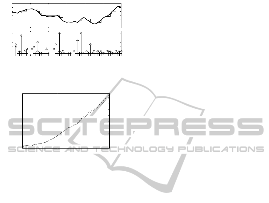
y[t], m[t]
samples
N
k
370
380
390
400 410 420
0
2
4
6
8
10
15
20
25
30
35
40
45
Figure 1: a) Measured (y[t]) and received outputs (m[t]) for
∆ = 2.0149. b) Intersampling periods (N
k
) for the three ap-
proaches: (’△’: KF, ’∗’: (18), ’◦’: (19)).
¯w
k¯xk
RMS
0 0.02 0.04 0.06 0.08
0.1
0.08
0.09
0.1
0.11
Figure 2: Achieved k˜x[t]k
RMS
as a function of the mean
value of w for ∆ = 2.0149 (’- -’: KF, ’–’: (19)).
the disturbance increases.
6 CONCLUSIONS
In this work, an observer codesign procedure for state
estimation over networks has been addressed using
the send-on-delta methodology (an output measure-
ment is transmitted only when the measured value has
changed more than ∆ with respect to the last transmit-
ted value). The design procedure consists of obtain-
ing both the observer gains and the maximum value
of ∆ that guarantees a prescribed state estimation er-
ror. The proposed observer is a gain-scheduling one
that applies a different gain depending on the avail-
ability of new measurements. The resulting closed
loop estimator dynamics has been obtained leading
to a linear discrete time switching system. Sufficient
conditions to assure the stability and a given level of
disturbance attenuation have been established under
the stated assumptions. Furthermore, a procedure to
obtain the maximum value of ∆ for a prescribed es-
timation error has been proposed. Two different al-
ternative approaches have been presented. In the first
one, a deterministic approach is used that guarantees
poly-quadratic stability and an H
∞
attenuation level,
assuming that no information about the derivative of
the output is known, leading to a value of ∆ that is
lower than the one obtained in other Kalman filter
based approaches, but resulting in a much lower com-
putational cost algorithm. In the second one, some
information about the output derivatives is assumed
to be known, and the optimization problem is formu-
lated in terms of the probabilities of output transmis-
sion, assuring mean square stability, and leading to
a value of ∆ that is larger than the one obtained in
other Kalman filter based approaches, i.e., leading to a
lower traffic over the network. Furthermore, the com-
putational cost of the resulting estimator is also much
lower than the Kalman filter one. A detailed example
has illustrated the validity of the approach compared
to the Kalman filter based approach.
REFERENCES
Dai, S.-L., Lin, H., and Ge, S. S. (2010). Scheduling-and-
control codesign for a collection of networked control
systems with uncertain delays. Control Systems Tech-
nology, IEEE Transactions on, 18(1):66 –78.
Gaid, M., Cela, A., and Hamam, Y. (2006). Optimal in-
tegrated control and scheduling of networked control
systems with communication constraints: application
to a car suspension system. Control Systems Technol-
ogy, IEEE Transactions on, 14(4):776 – 787.
Irwin, G., Chen, J., McKernan, A., and Scanlon, W. (2010).
Co-design of predictive controllers for wireless net-
work control. Control Theory Applications, IET,
4(2):186 –196.
Marck, J. and Sijs, J. (2010). Relevant sampling applied
to event-based state-estimation. In Sensor Technolo-
gies and Applications (SENSORCOMM), 2010 Fourth
International Conference on, pages 618 –624.
Miskowicz, M. (2006). Send-on-delta concept: An event-
based data reporting strategy. Sensors, 6(1):49–63.
Nguyen, V. H. and Suh, Y. S. (2007). Improving estima-
tion performance in networked control systems apply-
ing the send-on-delta transmission method. Sensors,
7(10):2128–2138.
Nguyen, V. H. and Suh, Y. S. (2008). Networked estimation
with an area-triggered transmission method. Sensors,
8(2):897–909.
Nguyen, V. H. and Suh, Y. S. (2009). Networked esti-
mation for event-based sampling systems with packet
dropouts. Sensors, 9(4):3078–3089.
Staszek, K., Koryciak, S., and Miskowicz, M. (2011). Per-
formance of send-on-delta sampling schemes with
prediction. In Industrial Electronics (ISIE), 2011
IEEE International Symposium on, pages 2037 –2042.
Suh, Y. S., Nguyen, V. H., and Ro, Y. S. (2007). Mod-
ified Kalman filter for networked monitoring sys-
tems employing a send-on-delta method. Automatica,
43(2):332 – 338.
Wang, X. and Lemmon, M. (2009). Self-triggered feedback
control systems with finite-gain stability. Automatic
Control, IEEE Transactions on, 54(3):452 –467.
ICINCO2012-9thInternationalConferenceonInformaticsinControl,AutomationandRobotics
504
