Nonlinear Deterministic Methods

for Computer Aided Diagnosis in Case of Kidney Diseases

Andreea Udrea, Mihai Tanase and Dumitru Popescu

Department of Automatics, University Politehnica of Bucharest, Bucharest, Romania

Keywords: Computer Aided Diagnosis, Nonlinear Deterministic Methods, CT Images.

Abstract: This paper proposes a set of nonlinear deterministic methods derived from chaos theory that can serve as

computed aided diagnosis tools for kidney diseases based on computer topographies (CT). These procedures

target the classification of the analyzed tissue samples in normal, malign and benign affected and also

enhanced visualization of the CT images. The classification methods consist in estimating the fractal

dimension of the kidney tissue and, respectively, the correlation dimension of the attractor obtained from the

spatial series associated to the kidney image. The enhanced visualization method associates a fractal map to

the analysed image. The methods are tested on 120 CTs presenting normal and modified tissue. The degree

of trustworthiness of the methods while dealing with classifications is discussed based on statistical results

and samples of fractal maps associated to the images are also presented.

1 INTRODUCTION

In order to increase the life expectancy and improve

the overall quality of life for patients with kidney

diseases, a critical stage in the medical process is to

employ a suitable protocol for delivering the

diagnostic, establish a treatment and, when needed,

to design an appropriate follow up procedure.

Usually, the first investigations and the follow up

consist in noninvasive or minimally invasive

procedures, in order to obtain the biological data for

proposing an accurate diagnostic. In this context,

any improvement in interpreting the patient’s data is

highly important.

When considering such data, at least two main

problems of tremendous importance have to be

solved: capturing and storing the considered medical

signals, on one hand and, on the other hand,

analyzing and interpreting the stored signal. In order

to capture 2D signals of the kidneys the most used

procedure is computer tomography (CT). The

obtained signals (grey level images) are usually

highly nonlinear, rather noisy and due to close

values of radio densities of the tissues, sometimes

difficult to interpret.

Analysis and interpretation of the captured

medical signals is almost exclusively subjected to

the human diagnosis expertise and experience. In the

last decade, a lot of effort was made to create

automatic analysis and diagnosis tools for aiding the

medical act. Nowadays, automatic diagnostic is still

a long term goal to be achieved, but Computer-

Aided Diagnosis (CAD) systems design seems

possible. This is confirmed by all major medical

imaging companies increasing interest in developing

CAD systems. Three signal processing operations

are closely related to CAD topics: filtering,

segmentation and quantification of analyzed

features. Enhanced visualization is another

important aspect, especially in the context of kidney

CT images presenting benign affected tissue.

The main goal of this paper is to present a series

of new or improved nonlinear methods that can aid

the medical diagnostic in the case of kidney diseases

and can be included in a CAD system. These

methods are derived from nonlinear time series

analysis and fractal geometry, both branches of

chaos theory. Their primary goal is to analyze the

kidney CT images and to decide if the presented

tissue is normal, malign affected, benign affected

and also to try differentiating between types of

benign diseases and malignancy stages. Where these

classification attempts prove limitations, enhanced

visualization procedures are offered as support.

The paper is organized in four chapters. In what

follows the nonlinear deterministic methods to be

used are presented and the results obtained by

employing them to the analysis of CTs are

511

Udrea A., Tanase M. and Popescu D..

Nonlinear Deterministic Methods for Computer Aided Diagnosis in Case of Kidney Diseases.

DOI: 10.5220/0004039405110516

In Proceedings of the 9th International Conference on Informatics in Control, Automation and Robotics (ICINCO-2012), pages 511-516

ISBN: 978-989-8565-21-1

 2012 SCITEPRESS (Science and Technology Publications, Lda.)

statistically analyzed. For this study, a series of 120

CT images were used: fifty of them contain malign

modified kidney tissue, fifty images present normal

kidney tissue and the rest of twenty are organised in

four images groups of benign affections. In the end

conclusions are summarized.

2 THE PROPOSED NONLINEAR

DETERMINISTIC METHODS

FOR CAD

Nonlinear time series analysis (NTSA) and fractal

analysis, as branches of chaos theory, provide useful

methods for the characterization of mono and multi

variable signals (like time series and images).

2.1 Attractor’s Correlation Dimension

Estimation Method for the CT

Image Associated Time Series

Typically, the NTSA deals with series that are sets

of values of a single variable function, usually

measured as function of time (dynamic features).

Nonlinear methods have been developed in the past

20 years, being motivated by the concept of

deterministic chaos, which is proved to exist within

many real systems in biology, medicine, chemistry,

physics and electronics. The studied time series in

medicine and biology are: recordings of the

electrical activity – electrocardiograms (EKG),

electroencephalograms (EEG) and physiological

parameters – blood pressure, pulse, and breathing

rate. Here are some applications with important

results of NTSA: diagnosis and control of cardiac

arrhythmia and ventricular fibrillations prediction

(Perc, 2005); characterization of sleep stages

(Rajendra, 2005); evaluation of variations in brain

functioning for psychical processes characterization

(Mekler,2008; Pritchard and Duke 1995);

characterization of anesthesia state (Widman, 2000).

The proposed NTSA derived method is based on

the invariant measure of a chaotic dynamical system:

the correlation dimension of the system’s attractor.

By investigating time series, one can observe the

behavior and properties of dynamical systems, in our

case of different physiological parameters.

From the mathematical point of view, there is a

formalism to describe the time series features. Let

the real valued map F :M →R be a measure on the

state space of some discrete dynamical system T

providing data in M. If s>0 is a fixed delay

(assigned to some sampling period) and x is a fixed

state, then a time series is a sequence of

measurements like the following:

F (T(t,x)), F (T(t + s,x)), F (T(t + 2s,x)),

…, F (T(t + (N −1)s,x))

(1)

for any starting instant t . Note that the state changes

too during the time series acquisition. The samples

of time series are often simply denoted by x

, x

t+1

t+2

, … .In context of medical signals, these time

series are measurement (like EEG, EKG) performed

on some patient (represented here by the system T ).

The acquisition rate and the length of the

measurement depend on the type of investigated

parameter. One can reconstruct the attractor of a

dynamical system from the time series generated by

the system, by using the Taken’s Embedding

Theorem (Taken, 1981) and computing the

correlation dimension of the attractor in order to

geometrically characterize it. The correlation

dimension d

is calculated using the following

recipe:

ln ( )

() , 0 lim

εεε

→

=→⇒=

(2)

where C(ε ) is the correlation integral defined below:

() lim ( | |)

CHyy

εε

→∞

=−−

∑

(3)

and: H is the Heaviside step function (which returns

either the unit value for non negative arguments or

null value otherwise), ε is the accepted distance

between points, y

is a point in the embedded phase

space constructed from a single time series,

according to Taken’s theorem, i.e:

=(x

i+s

i+2s

,…x

i+(dE-1)

s), s is the delay, d

is the

dimension of the embedding space where the

attractor resides, N is the number of embedding

vectors. So, C(ε ) gives the proportion of number of

points couples in the embedding space with the

Euclidian distance less than a specified small

threshold ε .

In pathology (especially in case of CT, RM

images and frozen tissues samples), one deals with

static (invariant) structures. In this case,

measurements are taken with respect to the one-

dimensional spatial axis, instead of temporal axis. In

this context we propose a method for reconstructing

the attractor from a CT image an associate to it a

specific d

In order to perform nonlinear analysis on a CT

normal or modified tissue image, a series of steps

must be made.

ICINCO2012-9thInternationalConferenceonInformaticsinControl,AutomationandRobotics

512

First, from a CT slice, the region containing the

tissue to be analyzed must be isolated; a matrix

containing values of each pixels shade is obtained

(the value can vary between 0 and 255

corresponding to different shades of grey; 0 stands

for black and 255 for white). The time (spatial)

series is generated in the following manner: the

matrix resulting from the original image is cut in

horizontal strips of 1, 2, 4, 8, … pixels, with respect

to the initial image dimension and precision; all

strips are put together one after another and generate

one single strip associated to the image; the time

(spatial) series - x(t) - is generated by computing

either the mean value or the maximal (dominant)

value of each column of pixels within the strip.

As result of this procedure, the time (spatial)

series associated to the section of the analyzed tissue

is obtained. For this study, since the analyzed CT

regions are not extremely large, a 1-pixel strip was

associated to each original image, this way not

altering the information provided by the image.

Having the associated series, the next step of the

procedure implies calculating the correlation

dimension of the attractor. This value is the

discrimination criterion.

However, in practical applications, in order to

determine the dimension of an attractor, we cannot

directly use the above formulae for d

due to the

following aspects: limited time series; noisy time

series; unknown fractal dimension of the attractor;

for different s - delay values different results due

autocorrelations; unknown d

– leading to time

correlations when reconstructing the series in a

embedding space with unsuitable dimension; time

series with the first part of data not on the attractor.

The delay or lag value -s- used to create the

delayed embedding must be properly chosen (Kantz

and Schreiber, 2003). A small value of the delay

generates correlated vector elements, while large

delay values yield to uncorrelated data and a random

distribution in the embedding space. The delay can

be chosen with good results as the moment of time

where the autocorrelation function of the

reconstructed series decays to 1/e of its initial value:

() (1)(1 1/)

NRN e

<−

(4)

Generally, the lag value is found between 4 and

10, while the used search interval is [1, 20].

The minimum allowed embedding dimension is

the dimension where the number of so called false

nearest neighbours drops under a certain percent. A

false neighbour is a point that under a certain higher

dimensional embedding is projected near a point that

in the previous embedding is not in its vicinity.

In order to implement this procedure, each point

of the delayed series is tested by taking its closest

neighbour in d

dimensions, and computing the ratio

of the distances between these two points in d

dimensions and in d

dimensions. If this ratio is

larger than a certain threshold th, the neighbour is

false (this threshold is taken large enough to take in

consideration points that exponential diverge due to

deterministic chaos):

id jd

−

(5)

where ||.|| is the Euclidian distance.

The percentage of false neighbours is computed

over a range of embedding dimensions (d

between 2

and 15) until it reaches a value less than a specified

limit; otherwise it considers the minimal obtained

value.

Once a proper delay and a minimum allowed

embedding dimension are determined, the

correlation dimension is calculated over a range of

different

- values and embedding dimensions

higher than the first assuring a decreased number of

false neighbours.

The d

differs from one embedding dimension to

another due to the noise in the data, but there is a

particular region, usually called the scaling region

where d

stabilizes (Kantz and Schreiber, 2003).

This is the interval where a mean value for the

correlation dimension of an attractor is calculated.

2.2 The Box-Counting Dimension

Estimation Method

Fractal analysis methods are used for the description

and quantization of geometric features of irregular

forms and patterns. Its most known tool is the fractal

dimension used to provide information on the

irregularity of an object contour or self-similarities

of a texture, which associates to some pathology as

well. It was applied for the study of medical systems

and subsystems at microscopic and macroscopic

scale, fracture analysis or texture classification

(Peitgen, 1992). The simplest medical application

consists in the morphological analysis of a structure

(for example, the lung network of arteries and

veins). This analysis of irregularities can be applied

in a similar manner on different forms, like the

delimitation between normal and affected tissue,

lesions, and tumors.

Here are some examples of fractal analysis

results in medicine and biology: classification in

pathology (Bassingthwaighte, 1994; Dobrescu si

NonlinearDeterministicMethodsforComputerAidedDiagnosisinCaseofKidneyDiseases

513

Vasilescu, 2004) and physiology (Luzi, 1999), tumor

growth description (Landini, 1998). The box

counting method provides a measure of fractal

dimension d

estimated for texture or contour.

The d

, derived from the Hausdorff coverage

dimension, is given by the following approximation:

()

log ( )

lim

log 1/

→

(6)

where: - N(s) is the number of squares with side

length s that contain information when grid covering

the image.

Relation (6) is the equation of the slope d

, of the

regression line associated to the points (log(N(s),

log(1/s)) for different values of the square’s side – s

of the covering grid..

The standard Box-Counting algorithm assumes

to determine the d

in accordance with the

dependence of the texture upon the used scale factor.

It consists transforming the grey scale image in

binary image, successively covering it with a grid of

squares of equal sides (2, 2

, 2

, ..) and counting each

time the squares that contain some part of the

analyzed object. The points of coordinates

(log(N(s)), log(1/s)) are approximately positioned in

a line and its slope is the fractal dimension in “box-

counting” sense.

To exemplify how the algorithm is used, we’ll

consider the image of a kidney (Figure 1. a)) from

which we’ll extract a binary version by neglecting all

the pixels over a certain threshold (Figure 1. b)).

a) b) c)

Figure 1: a) The original image; b) binary image

c) extracted contour.

Next, we’ll apply the box-counting algorithm,

described above, for different scale values s.

This method can be also used to determine the

self similarities of an object contour (Figure1 c)), but

in our case, due to the fact that the kidney capsule is

not necessary affected, the texture is more important.

A general problem of this method is the use of an

ad hoc threshold when creating the binary image.

This fact leads to incomplete or “noisy” object in the

binary image and sometimes importantly affects the

fractal dimension value.

2.3 Weighted Box-Counting Dimension

for Image Enhancement

This algorithm is based on the fact that in the CT

images a higher density of the tissue is equivalent to

lighter gray. Our idea was to associate to every pixel

a weight proportional to its gray level. We resume

the essential of the algorithm below.

Let us consider an image. We cover the image

with square boxes as in the standard Box-Counting

algorithm. Let

s be the size of the box used in

covering at step

(therefore we have to compute

)(

sN at this step). Let ),( yx be the coordinate

of the upper-left corner of one of these boxes (let

this be the box

B ).

We now define

m as the maximum of the

weight values of the pixels contained in this box.

(7)

where

is the weight associated to the pixel at

(i,j) coordinates.

Let

rsmW += ]/[

, where if

ms |

then

r else 0=

r .

Therefore

∑

WsN )( .

Next, the computation formula for d

is the

similar to the one in the classical algorithm. We

shall refer to the number d

as the Weighted Box

Counting Dimension or WBCD. Let us consider an

image and let A be a pixel on it. Let K be a square

centered at A. By using the previous algorithm we

compute the WBCD of the square K and we

associate a color to the pixel A according to this

WBCD (the function which associates the color is a

key part of the algorithm). This way we obtain a

map of level lines (we shall refer to this map as the

Fractal Map or FM).

This leads to a classification of different tissues

according to the associated color. Different structures

must have different colors. The use of the FM in

diagnosis requires a database with sufficient images.

3 RESULTS AND STATISTICS

We start the analysis procedure by presenting the

statistical results obtained by using d

and d

ICINCO2012-9thInternationalConferenceonInformaticsinControl,AutomationandRobotics

514

classification methods. One hundred and twenty CT

images were analysed; they were divided into two

equal samples: containing normal tissue and half

modified tissue.

For the statistical analysis, descriptive and

comparison procedures were performed. For each

sample, the average, standard deviation, standard

skewness and standard kurtosis were computed.

In order to compare the samples the t test and

Kolmogorov-Smirnov test were performed.

In the case of d

both comparison tests show no

significant difference between the two distributions

at the 95.0% confidence level. So, the

trustworthiness of this classification is low.

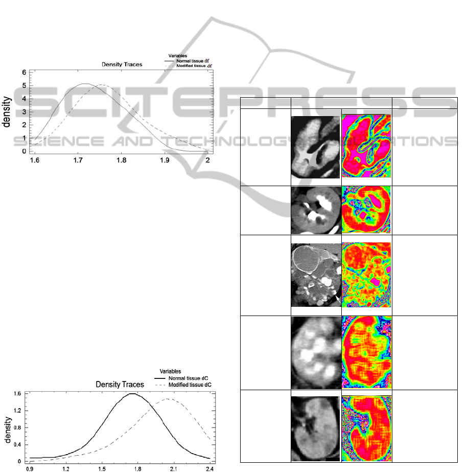
Figure 2: Comparison of density traces.

In the case of d

both comparison tests show

significant difference between the two distributions

at the 95.0% confidence level.

The average is 1.729 for the normal tissue and

respectively 1.974 for the modified tissue.

The 95.0% confidence interval for mean is

[1.6282,1.83155] for the normal tissue and

[1.87225,2.07725] for the modified tissue.

We conclude that the box-counting method is

using a certain threshold, this way loosing some

information on the tissue texture while nonlinear

analysis is more precise and uses all the information

in the images. We recommend the use of the second

method for analyzing CT images.

Figure 3: Comparison of density traces.

We have also compared the results acquired

when the CT was taken with contrast substances and

without. In the second case, the d

values are smaller

because of a series of features that are not so visible

(blood vessels). The differences between the d

normal and modified tissue samples are smaller. So,

we suggest that this methodology is better to be used

with associated time series resulting from CT images

taken with contrast substances.

The second step in the analysis was to determine

the correlation dimension of the attractor for images

containing kidneys with benign affections.

The discrimination is obvious in the cases of

pyelonephritis (the resulted d

values being smaller

than in the case of normal tissue) and kidney

tuberculosis (with

values larger than in the case

of malign modified tissue).

Table 1: Benign modified tissue images, their fractal maps

and associated d

values.

Affection Image Enhanced d

Pyelone-

phritis

1.36(correspo

ndent d

for

healthy kidney

-1.85)

Medullary

sponge

kidney

1.91(1.86)

Polycystic

kidney

2.06 (1.9)

Kidney

tuberculos

is (renal

TB)

2.3(1.92)

Thrombosi

1.98(1.93)

The d

values for medullary sponge kidney

tissue and thrombosis affected kidney tissue are

generally a little bit larger than the ones for normal

tissue.

NonlinearDeterministicMethodsforComputerAidedDiagnosisinCaseofKidneyDiseases

515

The d

values for polycystic kidney tissue were

generally larger than the ones for normal tissue.

In the third column of the above table the kidney

CT image fractal map is presented.

The kidney border and affection specific aspects

like different types of tissue clusters and their

delimitation can be seen clearer.

Also, the different colours in the map identify

different formations, specific to the affection.

This method proved more useful than the

previous two in aiding the diagnostic in the case of

benign affected tissue.

We conclude that discrimination between these

benign affections can be done but needs a larger

database of images.

Further work will focus on enlarging the CT

images data base in order to provide more accurate

discrimination interval values for different types of

kidney affections.

4 CONCLUSIONS

The conclusions of the study on the selected set of

CT images are: there are significant differences

between the correlation dimension of the normal

tissue and the correlation dimension of the modified

tissue; significantly better results are obtained in the

case of CT images taken when contrast substances

are used. The proposed nonlinear method for

estimated the correlation dimension associated to a

CT image proved efficient for differentiating

between normal and modified kidney tissue while

the box-counting method failed in providing useful

results. The image enhancement method proved very

helpful when inconclusive classification was

obtained for benign tissue.

Future work aims at: enlarging the CT images

data base; creating the fractal model of the kidney,

measuring, where it is possible, the percentage of the

modified tissue in a kidney CT slice in order to

provide information on what is causing the increase

in d

(percentage of affected tissue or d

value of

modified tissue); determining the position of masses

in an affected organ when considering horizontal

slices and respectively reconstructed transversal

slices in that organ .

REFERENCES

Bassingthwaighte J. B., Liebovitch L. S., West B. J.,

1994. Fractal Physiology. Oxford University Press

Dobrescu R., Vasilescu C., 2004. Interdisciplinary

applications of fractal and chaos theory. Romanian

Academy Press, pp. 247-254, 2004

Luzi P., Bianciardi G., Miracco C., De Santi M.M., Del

Vecchio M., Alia L., Tosi P., 1999. Fractal analysis in

human pathology. Ann. N.Y. Acad. Sci. 879, 255-257

Landini G., 1998. Complexity in tumor growth patterns,

Fractals in Biology and Medicine. Birkhäuser Verlag,

pp. 268-284

Kantz H., Schreiber T., 2003. Nonlinear time series

analysis, 2003. Cambridge University Press, 3

edition

Mekler A., 2008. Calculation of EEG correlation

dimension: Large massifs of experimental data.

Computer Methods and Programs in Biomedicine,

vol. 92, pp. 154-160

Peitgen H. O., Jurgens H., Saupe D., 1992. Chaos and

Fractals – New Frontiers of Science. Springer-Verlag

Perc M., 2005. Nonlinear time series analysis of human

electrocardiogram. In European Journal of Physics,

vol. 26, pp. 757-768.

Pritchard W. S., Duke D. W., 1995. Measuring chaos in

the brain: A tutorial review of EEG dimension

estimation. Brain Cognition, vol. 27, pp. 353-397

Rajendra U., Faust O., Kannathal N., Chua T.,

Laxminarayan S., 2005. Non-linear Analysis of EEG

Signals at Various sleep stages. In Computer Methods

and Programs in Biomedicine, vol. 80, pp. 37-45.

Takens F., 1981. Detecting strange attractors in fluid

turbulence. In Dynamical System andTurbulence,

Rand D. A., Young, L. S. (Eds), Lecture Notes in

Mathematics, Springer Verlag

Widman G., Schreiber T., Rehberg B., Hoerof A., Elger C.

E., 2000. Quantification of depth of anesthesia by

nonlinear time series analysis of brain electrical

activity. Physical Review E, no. 62, pp. 4898-4903

ICINCO2012-9thInternationalConferenceonInformaticsinControl,AutomationandRobotics

516