Trajectory Tracking Control of Nonholonomic

Wheeled Mobile Robots

Combined Direct and Indirect Adaptive Control using Multiple Models Approach

Altan Onat

and Metin Ozkan

Electrical & Electronics Engineering Department, Anadolu University, Iki Eylul Kampusu, Eskisehir, Turkey

Computer Engineering Department, Eskisehir Osmangazi University, Bati Meselik Kampusu, Eskisehir, Turkey

Keywords: Combined Direct and Indirect Adaptive Control, Trajectory Tracking Control, Nonholonomic Wheeled

Mobile Robots, Multiple Models Approach.

Abstract: This paper presents a novel methodology for the trajectory tracking control of nonholonomic wheeled

mobile robots using multiple identification models. The overall control system includes two stages. In the

first stage, a kinematic controller developed by using kinematic model provides the required linear and

angular velocities of the robot for tracking a reference trajectory. In the second stage, the required velocities

are taken as the inputs to an adaptive dynamic controller which uses multiple adaptive models for the

parameter identification. The proposed adaptive dynamic controller is developed using a combined direct

and indirect adaptive control approach where both prediction and tracking errors are used for identification.

Simulation results show the effectiveness of the proposed combined direct and indirect control scheme and

multiple models approach.

1 INTRODUCTION

Tracking control of a wheeled mobile robot (WMR)

is one of the most attractive research areas for the

several decades. Many WMR models and control

schemes have been presented. Generally, the aim of

such schemes is either to utilize a kinematic

trajectory tracking controller or to construct and

integrate kinematic and dynamic controllers to track

a desired trajectory. Yutaka et al. (1990) proposed a

control rule to determine reasonable linear and

rotational velocities for a stable tracking control. An

integrated kinematic controller and a torque

controller with a dynamic extension for a

nonholonomic mobile robot have been presented by

Fierro and Lewis (1995). Yun and Yamamoto

(1992) have studied feedback linearization of a

WMR and its dynamic system. A complete dynamic

model of a WMR which makes it suitable to

consider rotational and translational velocities as

control signals has been given by De La Cruz and

Carelli (2006).

For the tracking control of a WMR, there are also

adaptive control frameworks in literature. Felipe et

al. (2008) have proposed an adaptive controller to

guide a WMR during trajectory tracking. In this

study reference velocities are generated using a

kinematic model, and then these values are

processed to compensate for the robot dynamics. An

adaptive trajectory tracking controller for a

nonholonomic WMR with a nonlinear control law

based on input-output feedback linearization has

been proposed by Khoshnam et al. (2010). Cao et al.

(2011) has proposed an adaptive kinematic

controller to generate the command of velocity

based on backstepping method, and then Zhengcai et

al. (2011) has proposed adopting the reference

model with a dynamic adaptive controller. Similarly,

a new kinematic adaptive controller integrated with

a torque controller for the dynamic model of a

nonholonomic WMR has been proposed by

Takanori et al.(2000). Pourboghrat and Karlsson

(2002) has used adaptive control rules for the

dynamics level of nonholonomic WMRs with

unknown dynamic parameters and a fixed posture

backstepping technique for tracking a reference

trajectory and stabilization. Petrov (2010) has

proposed an adaptive dynamic based path control for

a differential drive mobile robot.

The studies previously mentioned provide the

schemes of trajectory tracking, but they did not

Onat A. and Ozkan M..

Trajectory Tracking Control of Nonholonomic Wheeled Mobile Robots - Combined Direct and Indirect Adaptive Control using Multiple Models Approach.

DOI: 10.5220/0004039800950104

In Proceedings of the 9th International Conference on Informatics in Control, Automation and Robotics (ICINCO-2012), pages 95-104

ISBN: 978-989-8565-22-8

 2012 SCITEPRESS (Science and Technology Publications, Lda.)

focus on the transient behaviour. However, when the

parameter errors are very large, the transient

response of the system may include unacceptably

large peaks. Although the system is asymptotically

stable, the adaptive control approach may be in

applicable for some systems due to the transient

peaks. To overcome this difficulty, the enhancement

of the transient response using multiple models and

switching has been proposed for the linear systems

by Narendra and Balakrishnan (1997). Some

approaches using multiple models and switching for

nonlinear systems have been presented in several

studies. Narendra and George (2002) have presented

a multiple model, switching and tuning methodology

which improves the transient performance for a class

of nonlinear systems. A novel approach which

makes use of multiple identification models and

switching based on direct adaptive control scheme

has been proposed by Cezayirli and Ciliz (2007).

Besides composite approach where both prediction

and tracking errors are used in a combined direct and

indirect adaptive control framework has been

studied by (Ciliz and Narendra, 1995) and (Ciliz and

Cezayirli, 2004). Ye (2008) has proposed a multiple

model adaptive controller for nonlinear systems in

parametric-strict-feedback form. An adaptive control

of a class of single-input single-output (SISO)

nonlinear systems considering transient performance

improvement by using multiple models and

switching has been considered by Cezayirli and Ciliz

(2006 and 2008). Ciliz and Narendra (1994), Ciliz

and Tuncay (2005) have used a scheme consisting of

multiple models, switching and tuning for the

adaptive control of robotic manipulators.

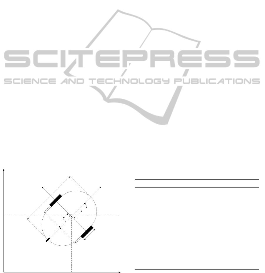
Figure 1: Nonholonomic WMR.

The purpose of this paper is to present an

integrated kinematic and dynamic controller for the

trajectory tracking of a WMR that includes

parametric uncertainties in the dynamics. A

composite approach, in which both prediction and

tracking errors are used in a combined direct and

indirect adaptive control framework with multiple

identification models and switching, is used. There

are a few works which make use of the multiple

models approach for the control of the WMRs. De

La Cruz et al. (2008) has proposed a switching

control for a novel tracking adaptive control of

WMRs. Another method that uses multiple models

of the robot for its identification in an adaptive and

learning control framework has been presented by

D’Amico et al. (2006).

2 KINEMATICS AND DYNAMICS

Consider the WMR model given by (1). The

parameters are given in Table 1 and the system is

shown in Figure 1. The system is subjected to m

constraints:

() (,) () ()

qq Cqqq Bq A q

τλ

+=+

&& & &

(1)

where

qR∈

is generalized coordinates,

∈

the input vector,

∈

is the vector of constraint

forces,

()

∈

is a symmetric positive-definite

inertia matrix,

(,)

Cqq R

∈

is coriolis matrix,

()

∈

is the input transformation matrix, and

()

∈

is the matrix associated with the

constraints.

Table 1: Model Parameters of WMR.

Parameter Description

r Driving wheel radius

2b Distance between two wheels

d Distance point Pc from point P0

a Distance from P0 to Pa

The mass of the platform without the driving

wheels and the rotors of the DC motors

The mass of each driving wheel plus the

rotor of its motor

The moment of inertia of the platform

without the driving wheels and the rotors of

the motors about a vertical axis through Pc

The moment of inertia of each wheel and the

motor rotor about the wheel axis

The moment of inertia of each wheel and the

motor rotor about a wheel diameter

Assuming that the velocity of

is in the direction

of x-axis of the local frame and there is no side slip,

and considering

[]

qxy

, the following

Castor

Wheel

ICINCO2012-9thInternationalConferenceonInformaticsinControl,AutomationandRobotics

constraint with respect to

is obtained

sin cos 0xy

ϕϕ

−=

(2)

By writing this constraint in matrix form, matrices

()

q and ()Sq are given by

[]

cos 0

() sin cos 0, () sin 0

Aq Sq

ϕϕ ϕ

⎡⎤

⎢⎥

=− =

⎢⎥

⎣⎦

(3)

Therefore, it can be written as

() () 0Aq Sq⋅= (4)

It is possible to write the kinematic equation of the

wheeled mobile robot motion in terms of the pseudo

velocities vector

()

vt R

−

∈

() ()

qSqvt=⋅

, (5)

where

[]

() () ()

vt vt t

∈

is made up of linear and

angular velocities. Taking the time derivative of (5)

() ()qSqvSqv=⋅+⋅

&& &

(6)

Next, by replacing (5) and (6) into (1),

multiplying the result by

and considering (4), the

following equation can be obtained

() ()() ()

vt Cvvt Bq

, (7)

where

SMS=

()

CSMSCS=+

and

SB=

By denoting

()

() ()()Mv t C v v t

, (8)

The matrices

and

are obtained as follows:





=

0

0

, 

=

0





−



 0



(9)

where 2

mm m=+ and

CmC W

IImdmb=+ + + .

There is a parametric vector

on dynamics that

satisfies

() ()() (, ,,)

vt Cvvt Y qqvv

&&&

, (10)

where the parameters

,1,,4

= K

are bounded and

defined as follows

123

, ,

mI md

θθθ

===

(11)

3 CONTROLLER DESIGN

3.1 Kinematic Controller

In the proposed control scheme, a kinematic

controller is used (Felipe et al., 2008). The design of

the kinematic controller is based on the kinematic

model of the WMR. The WMR’s kinematic model is

given by

cos sin

sin cos

ϕϕ

−

⎡⎤ ⎡ ⎤

⎡⎤

⎢⎥ ⎢ ⎥

⎢⎥

⎢⎥ ⎢ ⎥

⎣⎦

⎢⎥ ⎢ ⎥

⎣⎦ ⎣ ⎦

, (12)

where

are the coordinates of the point of

interest

, and the outputs. By assuming

[]

hxy=

cos sin

sin cos

avv

ϕϕ

ωω

−

⎡

⎤⎡ ⎤⎡⎤ ⎡⎤

== =

⎢

⎥⎢ ⎥⎢⎥ ⎢⎥

⎣

⎦⎣ ⎦⎣⎦ ⎣⎦

, (13)

where

cos sin

sin cos

ϕϕ

−

⎡

⎤

⎢

⎥

⎣

⎦

. (14)

The inverse of the matrix T is

cos sin

sin cos

ϕϕ

−

⎡

⎤

⎢

⎥

⎢

⎥

−

⎢

⎥

⎣

⎦

. (15)

Therefore, the inverse kinematics is given by

cos sin

sin cos

ϕϕ

⎡⎤

⎡

⎤⎡⎤

⎢⎥

⎢

⎥⎢⎥

⎢⎥

−

⎣

⎦⎣⎦

⎢⎥

⎣⎦

, (16)

and the proposed kinematic controller is given by

tanh

cos sin

sin cos

tanh

ref

yI y

ϕϕ

−

⎡⎤

⎛⎞

⎜⎟

⎢⎥

⎡⎤

⎝⎠⎡⎤

⎢⎥

⎛⎞

⎣⎦

⎢⎥

⎣⎦

⎜⎟

⎢⎥

⎝⎠

⎣⎦

(17)

Here,

xx=−

, and

yy y=−

are the current

position errors in the direction of

axis−

and

yaxis−

, respectively.

k >

and

k >

are the

gains of the controller,

R∈

, and

R∈

are

saturation constants, and

()

and

()

are the

current and desired coordinates of the point of

interest, respectively. The purpose of the kinematic

TrajectoryTrackingControlofNonholonomicWheeledMobileRobots-CombinedDirectandIndirectAdaptiveControl

usingMultipleModelsApproach

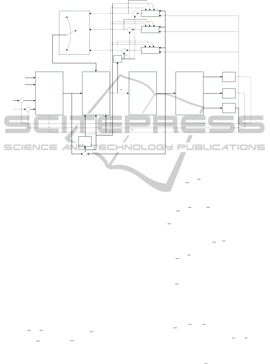
Figure 2: Block diagram of the control architecture.

controller is to generate the reference linear and

angular velocities for the dynamic controller as

shown in Figure 2.

3.2 Adaptive Dynamic Controller

A Proportional-Integral (PI) filtered velocity

tracking error signal is given as (Wilson and

Robinett, 2001)

eedt

∫

(18)

where

is a positive definite control gain and

velocity tracking error is defined as

evv=−

. (19)

where



















is the vector of the desired

linear and rotational velocities. Taking the derivative

of (18),

 =



+e



(20)

can be obtained. Considering (8) and adding the PI

filtered error terms yields

() ( , )

Ms C v s Y v v

θτ

+= −

(21)

(,) ( ) ()( )

dd d v d v

Yvv Mv e Cvv edt

θλ λ

=++ +

∫

(22)

To determine the control law and adaptive parameter

update rule, consider the following Lyapunov-like

function (Lewis et al., 2004)

VsMs

θθ

−

=+Γ

(23)

and differentiating the function with respect to time

TT T

VsMssMs

θθ

−

=++Γ

(24)

By taking

from (21) and adding to (24), the

following equation can be obtained

()

(,) ()

VsYvv Cvs

sMs

θτ

θθ

−

=−−

++Γ

. (25)

By choosing the control law

(,)

dd v

Yvv Ks

τθ

(26)

and adding (26) into the (25), the following equation

can be obtained

()

(,)

2 ( )

dd v

VsYvv sKs

sM Cvs

θθ

−

=−

+−+Γ

(27)

Reader should note that the matrix

2()

Cv−

is a

skew-symmetric matrix. By choosing the parameter

update rule as

()

(, ,) ( , )

fdd

Yqvv Yvvs

θτ

=−Γ +

∫

(28)

Kinematic

Controller

Dynamic

Controller

ref ref

WMR

Wheeled Mobile

Robot

, v

Kinematics

1/s

H(s)

Model 1

Model 2

Model N

1/s

∫

ICINCO2012-9thInternationalConferenceonInformaticsinControl,AutomationandRobotics

with an identification error model

(, ,)

Yq vv

τθ

∫

(29)

and inserting (28) into (27)

()

(,)

2 ( )

( , , ) ( , )

dd v

TT T

fdd

VsYvv sKs

sM Cvs

Yqvv Yvvs

θτ

−

=−

+−

+Γ−Γ +

∫

(30)

where

(, ,)Yq vv

∫

is the filtered regressor matrix

and

is the filtered torque term (Ciliz and

Narendra, 1994). Rearranging (29)

()

2()

( , , )

VsKssMCvs

Yqvv

θτ

=− + −

−

∫

(31)

may be obtained. By considering the identification

error model in (29) and adding into (31)

()

2()

(, ,) (, ,)

VsKssMCvs

Y q vvY q vv

θθ

=− + −

−

∫∫

(32)

may be obtained. For the proof of stability, the same

procedures should be followed (Lewis et al., 2004).

It should be noted that

is negative definite. It can

be stated that

in (23) is upper bounded and that

()

is a positive definite matrix it can be stated

that

and

are bounded. Standard linear control

arguments can be used to state that

and

∫

are

bounded. Since

,,,

ees

∫

are bounded it can be

shown that

and

are also bounded. The reader

should note that since

()

is lower bounded, it

can be stated that

is also lower bounded. Since

is lower bounded,

is negative definite and

is bounded, the Barbalat’s Lemma can be used to

state that

lim 0

→∞

(33)

which means that by Rayleigh-Ritz Theorem

{}

min

lim 0 or lim 0

Ks s

→∞ →∞

(34)

Using the standart linear control arguments the

following can be written

lim 0 and lim 0

→∞ →∞

∫

(35)

3.3 Adaptive Dynamic Controller with

Multiple Models

Identification models have the following structure

() ()() (, ,,)

jj j j

vt C vvt Y qqvv

τθ

=+ =

&&&

(36)

where

1, ,

N= K

denoting the parameter

estimate vector and

(,,,)Yqqvv

is the non-linear

regressor matrix. The regressor matrix common to

all models, but the parameter vector

has different

initializations chosen from a given compact

parameter set. Using the filtering technique

previously mentioned nonlinear regressor matrix

without acceleration signal can be obtained and will

be denoted as

(, ,)Yq vv

∫

. Each model is updated

using simple gradient algorithm as it is in single

model case:

((,,) (,))

jfdd

Yqvv Yvvs

θτ

=−Γ +

∫

(37)

based on the error model which is defined as,

(, ,)

jj j

Iff j

eYqvv

τττ θ

==−=

∫

(38)

where

is the filtered torque prediction error.

(,)

Yvv

is the regressor matrix common to all

models which is given in (22). The torque vector

jth

identification model is given as:

(,)

jddjv

Yv v Ks

τθ

. (39)

Adding the equations and (21) into (8), the closed

loop dynamics can be obtained as:

() ( ) ()( )

jj v jd jdv

sCvsKs Mv e Cvv e

λλ

++=++ +

∫

(40)

which can further be written as

() ( , )

jj v ddj

Ms C vs Ks Y v v

++=

(41)

At any instant, the identification errors of the

models are available, but only one of the torque

vectors

is chosen as the input to the WMR.

In order to choose a switching criterion, first a

permissible switching sequence and a switching rule

must be given (Ciliz and Narendra, 1994 & 1995). A

finite or infinite sequence

∈ RTT

is defined as a

switching sequence if

0T =

and

iT T

∀<

Additionally, if there is a number

min

0T >

such that

1min

iT T T

∀−≥

, then the sequence is called

permissible switching scheme.

A switching rule is a function of time that takes

values in the set

1, ,

is constant in

[

)

and

is continuous from right. In other words, a function

(): 1, ,ht R N

→ K

is called switching rule, if there

exists a switching sequence

such that if

[

)

tTT

∈

for some

i <∞

, then

() ( )

ht hT=

. With

this definition torque input in (21) can be defined as:

TrajectoryTrackingControlofNonholonomicWheeledMobileRobots-CombinedDirectandIndirectAdaptiveControl

usingMultipleModelsApproach

()

( ) ( ) 0.

ttt

ττ

=≥

(42)

The torque vector combined with a permissible

switching rule given as

()

() 2

(,)

ht d d j v

Yvv Ks

τθ

(43)

For the proof of stability, the same procedure will be

followed as in the single model case. The additional

requirement is that under any permissible switching

rule, all signals should remain bounded. We have a

Lyapunov-like function

jjjj

VsMs

θθ

−

=+Γ

(44)

The derivative of (44) can be obtained as in the

following equation

()

2()

(, ,) (, ,)

jv jj

VsKssMCvs

YqvvYqvv

θθ

=− + −

−

∫∫

(45)

is negative definite. It can be stated that

(44) is upper bounded and that

()

is a positive

definite matrix, it can be stated that

and

are

bounded. Standard linear control arguments can be

used to state that

and

∫

are bounded. Since

,,,

ees

∫

are bounded it can be shown that

and

are also bounded. The reader should note that

since

()

is lower bounded, it can be stated that

is also lower bounded. Since

is lower

bounded,

is negative definite and

is bounded,

the Barbalat’s Lemma can be used to state that

lim 0

→∞

, (46)

which means that by Rayleigh-Ritz Theorem

{}

min

lim 0 or lim 0

Ks s

→∞ →∞

==. (47)

Using the standard linear control arguments as in

single model case the following can be written

lim 0 and lim 0

→∞ →∞

∫

. (48)

3.4 Proof of Stability for the Kinematic

Controller

In order to understand the rest of the proof, the

reader may read (Martins et al., 2008). By

considering (13) and (14):

tanh

⎡⎤

⎛⎞

⎢⎥

⎜⎟

⎡⎤

⎝⎠

⎡⎤

⎢⎥

⎛⎞

⎣⎦

⎢⎥

⎜⎟

⎢⎥

⎝⎠

⎣⎦

(49)

One can see that the error vector

can also be

written as

, where

is the velocity tracking error

and matrix

T is defined before. Rewriting (49)

() ,

tanh

()

tanh

hLh Te

⎡

⎤

⎛⎞

⎢

⎥

⎜⎟

⎡⎤

⎝⎠

⎢

⎥

⎢⎥

⎢

⎥

⎛⎞

⎣⎦

⎢

⎥

⎜⎟

⎢

⎥

⎝⎠

⎣

⎦

(50)

Now considering Lyapunov candidate function

and its derivative

()

Vhh

VhhhTeLh

== −

%% % %

(51)

and a sufficient condition for

0V <

can be

expressed as

()

hLh hTe>

%% %

(52)

For small values of the control error h

following

can be written

() ,

xy xy

Lh K h K

⎡⎤

≈=

⎢⎥

⎣⎦

(53)

Now the sufficient condition for

0V <

can be

written as

min( , ) ,

min( , )

hK h hTe

kk h hTe

%%%

(54)

It is shown that

tend to zero as t →∞, which

implies that condition in (43) is verified for any

value of h

. Thus,

() 0ht →

as t →∞.

3.5 Switching Criterion

A cost function is considered in the form

()

() () () () ()

jj j j

TtT

jI I I I

t etGet e etGetd

λτ

−−

∫

(55)

where

is the cost function of the j

model,

ICINCO2012-9thInternationalConferenceonInformaticsinControl,AutomationandRobotics

100

the identification error associated with the j

model,

GG R

∈

are positive (semi)-definite weight

matrices and

≥

is a scalar forgetting factor.

is denoted as the cost function of the current model.

() ()

Jt Jt>

with defined switching sequence, it

means that adaptive model must be switched to the

model according to the switching criterion.

4 SIMULATIONS

In the simulations, the WMR should track an eight-

shaped trajectory given by

()

sin 2 ,

sin

rg r

xR t

yyR t

(56)

where

2.5

x =

5.5

y =

0.04

and

7.5R =

Initially robot

2x =

and

6.5y =

and robot has

zero velocities and

=−

The parameters of the WMR are taken as

0.0025 .

Kg m=

15.625 .

Kg m=

0.15rm=

0.75bm=

0.3 am=

0.3dm=

0.1

mKg=

0.005 .

Kg m=

K =

(10,10)diag

(2,2,2)diagΓ=

k =

I =

. The switching

sequence has a time step of 5 ms.

The real values of the unknown parameters are

[38 19.95 10.8]

= , and the initial estimates for

the parameters are

[20 7 3]

In order to show effectiveness of the developed

solution ten identification model has been chosen as









29 11 5





, 







32 14 7













35 17 9





, 







38 20 11













41 23 13





, 







44 26 15













47 29 17





, 







50 32 19













53 35 21





, 







56 38 23





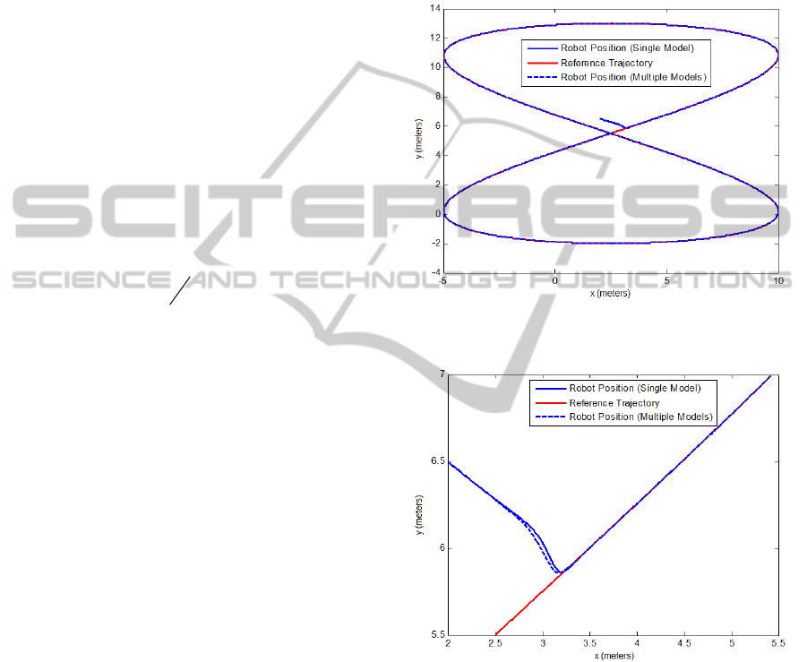
It can be seen from the figures that proposed control

approach enhances the performance of both velocity

tracking and trajectory tracking. In Fig. 3, there is a

trajectory tracking results for both single model and

multiple model cases. The controller provides the

reference trajectory tracking with a similar

performance for two cases. However, if one focus on

the trajectories for the first five seconds as seen in

Fig. 4, he can see the differences. Also, Fig. 5

shows the tracking errors on the x and y axis. In Fig.

6 and 8, there are linear and rotational velocity

errors, respectively. In order to show the

enhancement of the transient behaviour, Fig. 7 and 9

shows the linear and rotational errors for the first 5

seconds of the simulation. Similarly, Fig. 10-13

show the results for the integral of the linear and

rotational velocities. Fig. 14 shows the switching

between models during the simulation.

Figure 3: Robot position in single model case and multiple

model case vs. Reference Trajectory.

Figure 4: Robot position in single model case and multiple

model case vs. reference trajectory (five seconds to see the

effect).

TrajectoryTrackingControlofNonholonomicWheeledMobileRobots-CombinedDirectandIndirectAdaptiveControl

usingMultipleModelsApproach

101

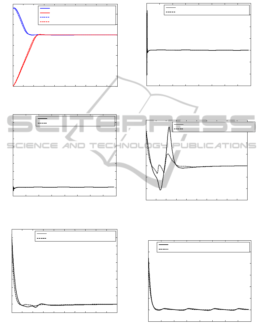
Figure 5: Position Errors on the x and y axis.

Figure 6: Linear velocity tracking error in single model

case and multiple models case.

Figure 7: Linear velocity tracking error in single model

case and multiple models case (five seconds to see the

effect).

Figure 8: Rotational velocity tracking error in single

model case and multiple models case.

Figure 9: Rotational velocity tracking error in single

model case and multiple models case (five seconds to see

the effect).

Figure 10: Integral of linear velocity tracking error in

single model case and multiple models case.

0 0.5 1 1.5 2 2.5 3 3.5 4 4.5 5

-1

-0.8

-0.6

-0.4

-0.2

0.2

0.4

0.6

Tim e

Position errors on the x and y axis

Position Error on the X-Axis (Single Model)

Position Error on the Y-Axis (Single Model)

Position Error on the X-Axis (Multiple Models)

Position Error on the Y-Axis (Multiple Models)

0 20 40 60 80 100 120 140 160

-0.2

0.2

0.4

0.6

0.8

1.2

1.4

1.6

1.8

Time

Tracking error1

Linear Velocity Tracking Error (Single Model)

Linear Velocity Tracking Error (Multiple Models)

0 0.5 1 1.5 2 2.5 3 3.5 4 4.5 5

-0.2

0.2

0.4

0.6

0.8

1.2

1.4

1.6

1.8

Tim e

Tracking error1

Linear Velocity Tracking Error (Single Model)

Linear Velocity Tracking Error (Multiple Models)

0 20 40 60 80 100 120 140 160

-0.6

-0.4

-0.2

0.2

0.4

0.6

0.8

Tim e

Tracking error2

Rotational Velocity Tracking Error (Single Model)

Rotational Velocity Tracking Error (Multiple Models)

0 0.5 1 1.5 2 2.5 3 3.5 4 4.5 5

-0.6

-0.4

-0.2

0.2

0.4

0.6

0.8

Tim e

Tracking error2

Rotational Velocity Tracking Error (Single Model)

Rotational Velocity Tracking Error (Multiple Models)

0 20 40 60 80 100 120 140 160

-0.05

0.05

0.1

0.15

0.2

0.25

0.3

Tim e

Integral of the Tracking error1

Integral of Linear Velocity Tracking Error (Single Model)

Integral of Linear Velocity Tracking Error (Multiple Models)

ICINCO2012-9thInternationalConferenceonInformaticsinControl,AutomationandRobotics

102

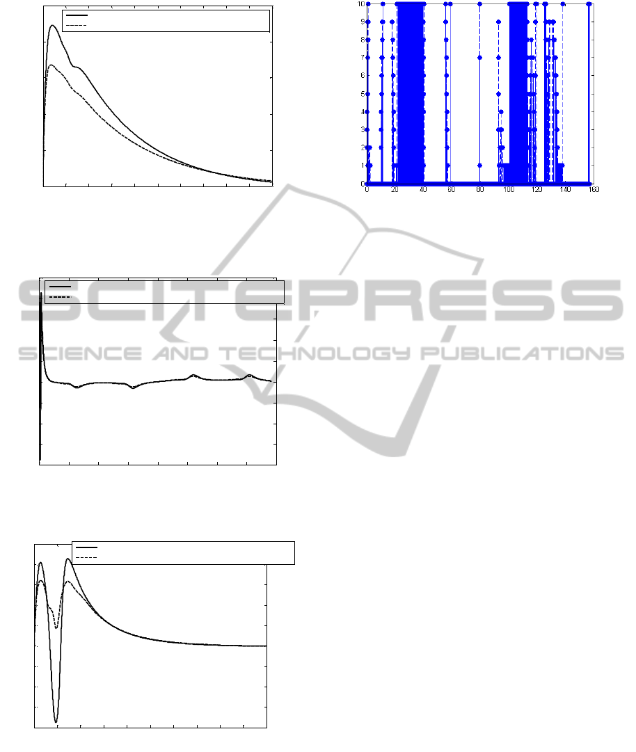
Figure 11: Integral of linear velocity tracking error in

single model case and multiple models case (ten seconds

to see the effect).

Figure 12: Integral of rotational velocity in single model

case and multiple models case.

Figure 13: Integral of rotational velocity in single model

case and multiple models case (ten seconds to see the

effect).

Figure 14: Switching between models.

5 CONCLUSIONS

An adaptive control algorithm with a multiple

models approach is proposed for the trajectory

tracking of a WMR. The controller uses a combined

direct and indirect adaptive control approach where

both prediction and tracking errors are used in

identification and switches between multiple models

of the WMR dynamics and the control input is

applied based on the model which closely describes

the WMR dynamics. This dynamic controller

provides fast velocity tracking under parameter

uncertainties. The proposed kinematic controller

provides the velocity profile needed for the

trajectory tracking of the WMR in Cartesian

coordinates. The stability of the overall control

system was proved. As a result, simulations show

that the proposed control system is applicable to the

WMR and it significantly enhances the transient

behavior during the trajectory tracking.

REFERENCES

Cezayirli, A., Ciliz, K., (2004). Multiple Model Based

Adaptive Control of a DC Motor Under Load

Changes., Proceedings of the IEEE International

Conference on Mechatronics.

Cezayirli, A., Ciliz, M. K., (2007). Transient Performance

Enhancement of Direct Adaptive Control of Nonlinear

Systems Using Multiple Models and Switching. IET

Control Theory Appl., 1(6), 1711-1725.

Cezayirli, A., Ciliz, M. K., (2008), Indirect Adaptive

Control of Non-Linear Systems Using Multiple

Identfication Models and Switching. International

Journal of Control, 81(9), 1434-1450.

Chen, W., Anderson, B. D. O., (2009). Multiple Model

Adaptive Control (MMAC) for Nonlinear Systems

with Nonlinear Parametrization. Joint 48

IEEE

0 1 2 3 4 5 6 7 8 9 10

0.05

0.1

0.15

0.2

0.25

Time

Integral of the Tracking error1

Integral of Linear Velocity Tracking Error (Single Model)

Integral of Linear Velocity Tracking Error (Multiple Models)

0 20 40 60 80 100 120 140 160

-0.08

-0.06

-0.04

-0.02

0.02

0.04

0.06

0.08

0.1

Time

Integral of the Tracking error2

Integral of the Rotational Velocity Tracking Error (Single Model)

Integral of the Rotational Velocity Tracking Error (Multiple Models)

0 1 2 3 4 5 6 7 8 9 10

-0.08

-0.06

-0.04

-0.02

0.02

0.04

0.06

0.08

0.1

Time

Integral of the Tracking error2

Integral of Rotational Velocity Tracking Error (Single Model)

Integral of Rotational Velocity Tracking Error (Multiple Models)

TrajectoryTrackingControlofNonholonomicWheeledMobileRobots-CombinedDirectandIndirectAdaptiveControl

usingMultipleModelsApproach

103

Conference on Decision and Control and 28

Chinese

Control Conference, Shangai, P.R. China.

Ciliz, K., Narendra, K. S., (1994). Multiple Model Based

Adaptive Control of Robotic Manipulators.

Proceedings of the 33

Conference on Decision and

Control. Lake Buena Vista, FL.

Ciliz, K., Narendra, K. S., (1995). Intelligent Control of

Robotic Manipulators: A Multiple Model Based

Approach. Intelligent Robots and Systems 95. 'Human

Robot Interaction and Cooperative Robots',

Proceedings.

Ciliz, K., Cezayirli, A., (2004). Combined Direct and

Indirect Control of Robot Manipulators Using

Multiple Models. Proceedings of the 2004 IEEE

Conference on Robotics, Automation and

Mechatronics, Singapore.

Ciliz, K., Tuncay, M. Ö., (2005). Comparative

Experiments with a Multiple Model Based Adaptive

Controller for SCARA Type Direct Drive

Manipulator. Robotica, 23(6), 721-729.

Ciliz, M. K., Cezayirli, A., (2006). Increased Transient

Performance for Adaptive Control of Feedback

Linearizable Systems Using Multiple Models.

International Journal of Control, 79(10), 1205-1215.

Ciliz, K., Cezayirli, A., (2006). Adaptive Tracking for

Nonlinear Plants Using Multiple Identification Models

and State-Feedback. IEEE Industrial Electronics,

IECON 2006 - 32nd Annual Conference.

De La Cruz, C., Carelli, R., (2006). Dynamic Modeling

and Centralized Formation Control of Mobile Robots.

IEEE Industrial Electronics, IECON 2006.

D’Amico, A., Ippoliti, G., Longhi, S., (2006). A Multiple

Models Approach for Adaptation and Learning in

Mobile Robots Control. Journal of Intelligent Robot

Systems, 47, 3-31.

De La Cruz, C., Carelli, R., Bastos, T. F., (2008).

Switching Adaptive Control of Mobile Robots.

Industrial Electronics, 2008, ISIE 2008, IEEE

International Symposium.

Fierro, R., Lewis, F. L., (1995). Control of a Nonholonomic

Mobile Robot: Backstepping Kinematics into

Dynamics. Proceedings of the 34

Conference on

Decision and Control. New Orleans, LA.

Fukao, T., Nakagawa, H., Adachi, N., (2000). Adaptive

Tracking Control of a Nonholonomic Mobile Robot.

IEEE Transactions on Robotics and Automation,

16(5), 609-615.

Gholipour, A., Yazdanpanah, M. J., (2003). Dynamic

Tracking Control of Nonholonomic Mobile Robot

with Model Reference Adaptation for Uncertain

Parameters. European Control Conference

Cambridge, UK.

Islam, S., Liu, P. X., (2009). Adaptive Output Feedback

Control for Robot Manipulators Using Lyapunov-

Based Switching. The 2009 IEEE/RJS International

Conference on Intelligent Robots and Systems, St.

Louis, USA.

Kalkkuhl, J., Johansen, T. A., Lüdemann, J., (2002).

Improved Transient Performance of Nonlinear

Adaptive Backstepping Using Estimator Resetting

Based on Multiple Models. IEEE Transactions on

Automatic Control, (47)1, 136-140.

Kanayama, Y., Kimura, Y., Miyazaki, F., Noguchi, T.,

(1990). A Stable Tracking Control Method for an

Autonomous Mobile Robot. Robotics and Automation

International Conference. USA.

Lee, C. Y., (2006). Adaptive Control of A Class of

Nonlinear Systems Using Multiple Parameter Models.

International Journal of Control, Automation, and

Systems, 4(4), 428-437.

Martins, F. N., Celeste, W. C., Carelli, R., Sarcinelli-Filho,

M., Bastos-Filho, T., (2008), An Adaptive Dynamic

Controller for Autonomous Mobile Robot Trajectory

Tracking. Control Engineering Practice, 16, 1354-1363

Narendra, K. S., Balakrishnan, J., (1997). Adaptive

Control Using Multiple Models. IEEE Transactions on

Automatic Control, 42(2), 171-187.

Narendra, K. S., George, K., (2002). Adaptive Control of

Simple Nonlinear Systems Using Multiple Models.

Proceedings of the American Control Conference

Anchorage.

Park, B. S., Park, J. B., Choi, Y. H., (2011). Adaptive

Observer-Based Trajectory Tracking Control of

Nonholonomic Mobile Robots. International Journal

of Control, Automation, and Systems, 9(3), 534-541.

Petrov, P., (2010), Modeling and Adaptive Path Control of

a Differential Drive Mobile Robot. Proceedings of the

12th WSEAS International Conference on Automatic

Control, Modellig and Simulation.

Pourboghrat, F., Karlsson, M. P., (2002). Adaptive

Control Of Dynamic Mobile Robots with

Nonholonomic Constraints. Computers & Electrical

Engineering, 28(4), 241-253.

Shojaei, K., Shahri, A. M., Tarakameh, A., Tabibian, B.,

(2011). Adaptive Trajectory Tracking Control of a

Differential Drive Wheeled Mobile Robot. Robotica,

29(3), 391-402.

Wison, D. G., Robinett, R. D., (2001). Robust Adaptive

Backstepping Control for a Nonholonomic Mobile

Robot. IEEE International Conference on Systems,

Man, and Cybernetics.

Ye, X., (2008), Nonlinear Adaptive Control Using

Multiple Identification Models. Systems & Control

Letters, 3, 488-491.

Yun, X., Yamamoto, Y., (1992). On Feedback

Linearization of Mobile Robots. Department of

Computer & Information Science Technical Reports.

University of Pennsylvania.

Zhengcai, C., Yingtao, Z., Qidi, W., Adaptive Trajectory

Tracking Control for a Nonholonomic Mobile Robot.

Chinese Journal of Mechanical Engineering, 24(3), 1-7.

ICINCO2012-9thInternationalConferenceonInformaticsinControl,AutomationandRobotics

104