
Compensation of Tool Deflection in Robotic-based Milling
Alexandr Klimchik
1,2
, Dmitry Bondarenko
2,3
, Anatol Pashkevich
1,2
,
Sebastien Briot
2
and Benôit Furet
2,4
1
Ecole des Mines de Nantes, 4 Rue Alfred-Kastler, 44307, Nantes, France
2
Institut de Recherches en Communications et Cybernétique de Nantes, UMR CNRS 6597, Nantes, France
3
Ecole Centrale de Nantes, 1 Rue de la Noë, 44 321, Nantes, France
4
Université de Nantes, Quai de Tourville, 44035, Nantes, France
Keywords: Industrial Robot, Milling, Compliance Error Compensation, Dynamic Machining Force Model, Non-linear
Stiffness Model.
Abstract: The paper presents the compliance errors compensation technique for industrial robots, which are used in
milling manufacturing cells. under external loading, which is based on the non-linear stiffness model. In
contrast to previous works, it takes into account the interaction between the milling tool and the workpiece
that depends on the end-effector position, process parameters and cutting conditions (spindle rotation, feed
rate, geometry of the tool, etc.). Within the developed technique, the compensation errors caused by external
loading is based on the non-linear stiffness model and reduces to a proper adjusting of a target trajectory
that is modified in the off-line mode. The advantages and practical significance of the proposed technique
are illustrated by an example that deals with milling with Kuka robot.
1 INTRODUCTION
Currently, robots become more and more popular for
a variety of technological processes, including high-
speed precision machining. For this process, the robot
is subjected by external loading which caused by the
machining force. This force is generated by the inter-
action between the tool mounted on the robot end-
effector and the workpiece during the material re-
moval (Dépincé, 2006). It is a contact force and it is
distributed along the affected area of the tool cutting
part. To evaluate the influence and to analyze the ro-
bot behavior while machining, the cutting force
should be defined either experimentally or using accu-
rate mathematical model.
To evaluate the force caused by interaction be-
tween the tool and the workpiece, two approaches can
be used. The static approach allows computing the
average cutting force without any consideration of
dynamic aspect in machining system. This force
serves as an external loading of the robot. This ap-
proach is widely used in analysis of conventional ma-
chining processes using CNC machines (Altintas,
2000), where the stiffness is high. In contrast, robots
have relatively low structural stiffness. For this rea-
son, in the case of robotic-based machining, an addi-
tional source of dynamic displacements of the end-
effector with respect to the desired trajectory induced
by robot compliance may arise. Such behavior leads
to the variable contact between the machining tool
and the workpiece. Thus, the generated contact force
depends on the current position of the robot end-
effector on the trajectory. Consequently, the cutting
force cannot be evaluated correctly using the static
approach. In this case, the dynamic approach, which
will be used in the paper, is required. It is based on
computing of the force at each instant of machining
process that defines loading of the robot for the next
instant of processing. As a result, the dynamic aspect
of robot motion under such variable cutting force can
be examined for whole process.
Usually, in the robot-based machining this force
causes essential deflections that decrease the quality
of the final product. The problem of the robot error
compensation can be solved in two ways that differ in
degree of modification of the robot control software:
(a) by modification of the manipulator model,
which better suits to the real manipulator and is used
by the robot controller (in simple case, it can be lim-
ited by tuning of the nominal manipulator model, but
113
Klimchik A., Bondarenko D., Pashkevich A., Briot S. and Furet B..
Compensation of Tool Deflection in Robotic-based Milling.
DOI: 10.5220/0004040801130122
In Proceedings of the 9th International Conference on Informatics in Control, Automation and Robotics (ICINCO-2012), pages 113-122
ISBN: 978-989-8565-22-8
Copyright
c
2012 SCITEPRESS (Science and Technology Publications, Lda.)

may also involve essential model enhancement by
introducing additional parameters, if it is allowed by
a robot manufacturer);
(b) by modification of the robot control pro-
gram that defines the prescribed trajectory in Carte-
sian space (here, using relevant error model, the input
trajectory is generated in such way that under the
loading the output trajectory coincides with the de-
sired one, while input trajectory differs from the target
one).
Moreover, with regard to the robot-based machin-
ing, there is a solution that does not require
force/torque measurements or computations (Dépincé,
2006), where the target trajectory for the robot con-
troller is modified by applying the "mirror" technique.
An evident advantage of this technique is its applica-
bility to the compensation of all types of the robot er-
rors, including geometrical and compliance ones.
However, this approach requires carrying out addi-
tional preliminary experiments which are quite expen-
sive. So, it is suitable for the large-scale production
only. Another compensation methodology has been
proposed by Eastwood and Webb (Eastwood, 2010)
that was used for gravitational deflection compensa-
tion for hybrid parallel kinematic machines.
This paper focuses on the modification of control
program that is considered to be more realistic in
practice. This approach requires also accurate stiff-
ness model of the manipulator. From point of view of
stiffness analysis, the external and forces directly in-
fluence on the manipulator equilibrium configuration
and, accordingly, may modify the stiffness properties.
So, they must be undoubtedly taken into account
while developing the stiffness model. However, in
most of the related works the Cartesian stiffness ma-
trix has been computed for the nominal configuration
(Chen, 2000; Alici, 2005). Such approach is suitable
for the case of small deflections only. For the opposite
case, the most important results have been obtained in
(Kövecses, 2007; Tyapin, 2009; Pashkevich, 2011),
which deal with the stiffness analysis of manipulators
under the end-point loading.
Thus, to compensate errors caused by the machin-
ing process, it is required to have an accurate stiffness
model and precise cutting force model. In contrast to
the previous works, the compliance error compensa-
tion technique presented in this work is based on the
non-linear stiffness model of the manipulator (Pash-
kevich, 2011) and dynamic model of technological
process that generates the cutting force.
2 PROBLEM STATEMENT
For the compliance errors, the compensation tech-
nique must rely on two components. The first of them
describes distribution of the stiffness properties
throughout the workspace and is defined by the stiff-
ness matrix as a function of the joint coordinates. The
second component describes the forces/torques acting
on the end-effector while the manipulator is perform-
ing its machining task (manipulator loading).
The stiffness matrix required for the compliance
errors compensation highly depends on the robot
configuration and essentially varies throughout the
workspace. From general point of view, full-scale
compensation of the compliance errors requires es-
sential revision of the manipulator model embedded
in the robot controller. In fact, instead of conven-
tional geometrical model that provides inverse/direct
coordinate transformations from the joint to Carte-
sian spaces and vice versa, here it is necessary to
employ the so-called kinetostatic model (Su, 2006).
It is essentially more complicated than the geomet-
rical model and requires rather intensive computa-
tions that are presented in Section 3..
The dynamic behavior of the robot under the load-
ing
F caused by technological process can be de-
scribed as
CC C
+
+=M δtCδtKδtF
&& &
(1)
where
C
M is 66
×
mass matrix that represents the
global behavior of the robot in terms of natural fre-
quencies,
C
C is 66
×
damping matrix,
C
K is 66
×
Cartesian stiffness matrix of the robot under the ex-
ternal loading
F
, ,δt δt
&
and δt
&&
are dynamic dis-
placement, velocity and acceleration of the tool end-
point in a current moment respectively (Briot, 2011).
In general, the cutting force F
c
has a nonlinear na-
ture and depends on many factors such as cutting
conditions, properties of workpiece material and tool
cutting part, etc (Ritou, 2006). But, for given
tool/workpiece combination, the force F
c
could be ap-
proximated as a function of an uncut chip thickness h,
which represents the desired thickness to cut at each
instant of machining.
Hence, to reduce errors caused by cutting forces in
the robotic-based machining it is required to obtain an
accurate elasto-static model of robot and elasto-
dynamic model of machining process. These prob-
lems are addressed in the following sections taking
into account some particularities of the considered
application (robotic-based milling).
ICINCO2012-9thInternationalConferenceonInformaticsinControl,AutomationandRobotics
114
3 MANIPULATOR MODEL
3.1 Elasto-Static Model
Elasto-static model of a serial robot is usually de-
fined by its Cartesian stiffness matrix, which should
be computed in the neighborhood of loaded configu-
ration. Let us propose numerical technique for com-
puting static equilibrium configuration for a general
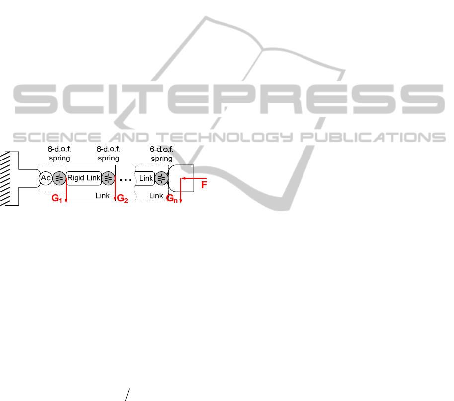
type of serial manipulator. Such manipulator may be
approximated as a set of rigid links and virtual
joints, which take into account elasto-static proper-
ties (Figure 1). Since the link weight of serial robots
is not negligible, it is reasonable to decompose it in-
to two parts (based on the link mass centre) and ap-
ply them to the both ends of the link. All this load-
ings will be aggregated in a vector
[
]
1
...
n
=GGG,
where
i
G is the loading applied to the i-th node-
point. Besides, it is assumed that the external load-
ing
F (caused by the interaction of the tool and the
workpiece) is applied to the robot end-effector.
Figure 1: VJM model of industrial robot with end-point
and auxiliary loading.
Following the principle of virtual work, the work
of external forces
,GF is equal to the work of inter-
nal forces
θ
τ caused by displacement of the virtual
springs
δθ
()
TTT
θ
1
δδδ
n
jj
j =
⋅+⋅=⋅
∑
GtFtτθ (2)
where the virtual displacements
δ
j
t can be comput-
ed from the linearized geometrical model derived
from
()
θ
δδ,1..
j
j
jn==tJθ , which includes the Jaco-
bian matrices
(
)
()
θ
,
j
j
=∂ ∂Jgqθθ with respect to
the virtual joint coordinates.
So, expression (2) can be rewritten as
()()
T() T() T
θθθ
1
δδδ
n
jn
j
j
=
⋅⋅+⋅⋅=⋅
∑
GJ θ FJ θτ θ (3)
which has to be satisfied for any variation of
δθ . It
means that the terms regrouping the variables
δθ
have the coefficients equal to zero. Hence the force
balance equations can be written as
()T ()T
θθ θ
1
n
jn
j
j
=
=
⋅+ ⋅
∑
τ JGJF (4)
These equations can be re-written in block-matrix
form as
(G)T (F)T
θθ θ
=
⋅+ ⋅τ JGJF (5)
where
(F) ( )
θθ
n
=JJ,
(G) (1) ( )
θθθ
T
TT
...
n
⎡⎤
=
⎣⎦
JJJ
,
T
TT
1
...
n
⎡
⎤
=
⎣
⎦
GGG
. Finally, taking into account the
virtual spring reaction
θθ
=⋅τ K θ , where
(
)
1n
θθθ
,...,diag=KKK, the desired static equilibri-
um equations can be presented as
(G)T (F)T
θθ θ
⋅
+⋅=⋅JGJFKθ (6)
To obtain a relation between the external loading
F and internal coordinates of the kinematic chain θ
corresponding to the static equilibrium, equations (6)
should be solved either for different given values of
F or for different given values of t . Let us solve the
static equilibrium equations with respect to the ma-
nipulator configuration
θ and the external loading
F
for given end-effector position
()
=tgθ and the
function of auxiliary-loadings
()
G θ
() ()
(G)T (F)T
θθ θ
;;⋅= + = =K θ JGJFt
g
θ GGθ (7)
where the unknown variables are
()
,θ F .
Since usually this system has no analytical solu-
tion, iterative numerical technique can be applied. So,
the kinematic equations may be linearized in the
neighborhood of the current configuration
i
θ
(
)
(
)( )
(F)
θ11
;
ii iii++
=+ ⋅−tgθ J θθ θ (8)
where the subscript '
i' indicates the iteration number
and the changes in Jacobians
(G) (F)
θθ
,JJ
and the auxil-
iary loadings
G are assumed to be negligible from
iteration to iteration. Correspondingly, the static
equilibrium equations in the neighborhood of
i
θ
may be rewritten as
(G)T (F)T
θ 1θ 1 θ
ii
+
+
⋅
+⋅=⋅JGJFKθ
. (9)
Thus, combining (8), (9) and analytical expression
for
1(G)T (F)T
θθ θ
()
−
=
⋅+ ⋅θ KJ GJ F, the unknown varia-
bles
F and θ can be computed using following itera-
tive scheme
CompensationofToolDeflectioninRobotic-basedMilling
115

()
()
()
()
1
(F) 1 (F)T
θθ
(F) (F) 1 (G)T
θθ θ
1(G)T (F)T
θθ
1
1
1θ1
·
i
ii i i
iii
θ
θ
+
+
+
−
−
−
+
−
=⋅⋅
−+−
=⋅+⋅
FJKJ
tgθ J θ JK J G
θ KJ GJ F
(10)
The proposed algorithm allows us to compute the
static equilibrium configuration for the serial robot
under external loadings applied to any point of the
manipulator and the loading from the technological
process.
3.2 Stiffness Matrix
In order to obtain the Cartesian stiffness matrix, let
us linearize the force-deflection relation in the
neighborhood of the equilibrium. Following this ap-
proach, two equilibriums that correspond to the ma-
nipulator state variables
(, ,)F θ t and
( δ , δ , δ )+++FFθθtt should be considered simul-
taneously. Here, notations
δF , δt define small in-
crements of the external loading and relevant dis-
placement of the end-point. Finally, the static equi-
librium equations may be written as
()
(G)T (F)T
θθ θ
;=⋅=⋅+⋅tgθ K θ JGJF (11)
and
()
()
()
()
()
()
T
(G) (G)
θθθ
T
(F) (F)
θθ
δδ
δδ δ
δδ
+= +
⋅+ = + ⋅ +
++ ⋅+
ttgθθ
K θθ JJ GG
JJ FF
(12)
where
θ
,,, ,tFGK θ are assumed to be known.
After linearization of the function
()g θ in the
neighborhood of the loaded equilibrium, the system
(11), (12) is reduced to equations
(F)
θ
(G) (G) (F) (F)
θθθ θθ
δδ
δδ δ δ δ
=
⋅= + + +
tJ θ
K θ JGJ G JFJ F
(13)
which defines the desired linear relations between
δt and δF . In this system, small variations of Jaco-
bians may be expressed via the second order deriva-
tives
(F) (F)
θθθ
δδ=⋅JHθ ,
(G) (G)
θθθ
δδ=⋅JHθ , where
(G) 2
θθ
1
2T
j
j
j
n
=
=∂ ∂
∑
HgGθ ,
(F
θθ
2)2T
=∂ ∂HgFθ . Al-
so, the auxiliary loading
G may be computed via
the first order derivatives as
δδ=∂ ∂ ⋅GGθθ
Further, let us introduce additional notation
(F) (G) (G)T
θθ θθ θθ θ
=++ ⋅∂∂HHH J Gθ
, which allows us to
present system (13) in the form
(F)
θ
(F)T
θθθθ
δδ
δ
⎡⎤
⎡
⎤⎡⎤
=⋅
⎢⎥
⎢
⎥⎢⎥
−+
⎣
⎦⎣⎦
⎣⎦
0J
tF
0 θ
JKH
(14)
So, the desired Cartesian stiffness matrices
C
K can
be computed as
(
)
1
(F) 1 (F)T
C θθ θθθ
()
−
−
=−KJKHJ (15)
Below, this expression will be used for computing of
the elasto-static deflections of the robotic manipula-
tor.
3.3 Mass Matrix
To evaluate dynamic behaviour of the robot under
the loading, in addition to the Cartesian stiffness ma-
trix
C
K it is required to define the mass matrix
C
M .
Comprehensive analysis and definition of this matrix
have been proposed in (Briot, 2011). Here, let us
summarise the main results that will be used further
in the error compensation technique.
Similar to the stiffness matrix, here physical prop-
erties defined by the mass matrix
C
M are constant in
the joint coordinates
θ
const
=
M and are defined by
the mass matrices
θi
M of all n links of the robot
θθ1 θn
( ,..., )diag
=
MMM. Assuming that link may be
approximated by a beam with a constant cross-
section, the mass matrix
θi
M can be computed as
θ 123456
(, , , , , )
i
diag a a a a a a
=
M (16)
where
1
/3
i
am
=
,
2
33 /140
i
am
=
,
3
33 /140
i
am= ,
4
/3
p
iii
aIL
ρ
= ,
5
8/15
y
iii
aIL
ρ
= ,
6
8/15
z
iii
aIL
ρ
= ,
i
m is physical mass of i-th link,
i
ρ
is density of i-th
link,
i
L is link length,
p
i
I
is the polar moment,
,
yz
ii
II
are the second moments of the area. Since the
mass matrix
θ
M is defined in the joint coordinates it
can be recomputed into the Cartesian coordinates
associated with the tool end-point using the Jacobian
matrix
θ
J (which depend on the robot configuration
q and computed with respect to virtual joint coordi-
nates
θ ) using following expression
θC θθ
T
=MJMJ (17)
Thus, using expressions (16) and (17) it is possible
to compute the mass matrix
C
M for a given robot
configuration
q .
ICINCO2012-9thInternationalConferenceonInformaticsinControl,AutomationandRobotics
116
4 MACHINING PROCESS
Let us obtain the model of the cutting force which de-
pends on the relative position of the tool with respect
to the workpiece at each instant of machining. As fol-
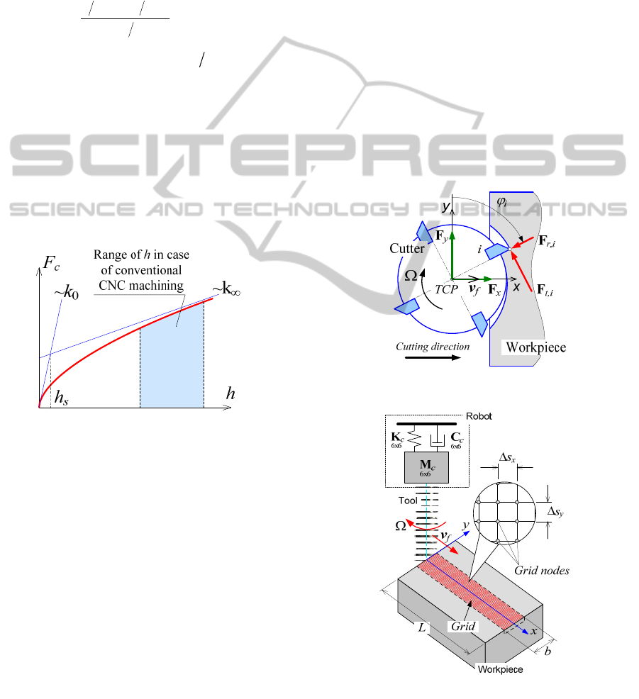
lows from previous works (Brissaud, 2008), for the
known chip thickness
h, the cutting force F
c
can be
expresses as
()
()
2
0
,0
1
ss
c
s
p
hh r hh
Fh k a h
hh
+
=≥
+
(18)
where
p
a is a depth of cut,
0
1rkk
∞
=< depends
on the parameters
k
∞
, k
0
that define the so called
stiffness of the cutting process for large and small
chip thickness
h respectively (Figure 2) and h
s
is a
specific chip thickness, which depends on the cur-
rent state of the tool cutting edge. The parameters
k
0
,
h
s
, r are evaluated experimentally for a given com-
bination of tool/working material. To take into ac-
count the possible loss of contact between the tool
and the workpiece, expression (18) should be sup-
plement by the case of
0h
<
as
Figure 2: Fractional cutting force model F
c
(h).
()
0, if 0
c
Fh h=< (19)
For the multi-edge tool the machining surface is
formed by means of several edges simultaneously.
The number of working edges varies during machin-
ing and depends on the width of cut. For this reason,
the total force
F
c
of such interaction is a superposition
of forces
F
c,i
generated by each tool edge i, which are
currently in the contact with the workpiece. Besides,
the contact force
F
c,i
can be decomposed by its radial
F
r,i
and tangential F
t,i
components (Figure 3). In ac-
cordance with Merchant’s model (Merchant, 1945),
the
t-component of cutting force F
t,i
can be computed
with the equation (18). The
r-component F
r,i
is related
with
F
t,i
by following expression (Laporte 2009)
,,ri r ti
F
kF= (20)
where the ratio factor
k
r
depends on the given
tool/workpiece characteristics.
It should be mentioned that in robotic machining it
is more suitable to operate with forces expressed in
the robot tool frame {
x,y,z}. Then, the corresponding
components
F
x
, F
y
(Figure 3) of the cutting force F
c
can be expressed as follows
,,
11
,,
11
cos sin
sin cos
zz
zz
nn
x
ri i ti i
ii
nn
yriitii
ii
FF F
FF F
ϕ
ϕ
ϕ
ϕ
==
==
=− +
=+
∑∑
∑∑
(21)
where
n
z
is the number of currently working cutting
edges,
φ
i
is the angular position of the i-th cutting
edge (the cutting force in
z direction F
z
is negligible
here). So, the vector of external loading of the robot
due to the machining process can be composed in
the frame {
x,y,z} using the defined components F
x
,
F
y
as F=[F
x
,F
y
,0,0,0,0]
T
.
Figure 3: Forces of tool/workpiece interaction.
Figure 4: Meshing of the workpiece area.
It should be stressed that the cutting force compo-
CompensationofToolDeflectioninRobotic-basedMilling
117
nents
F
r,i
, F
t,i
mentioned in equation (18),(20) are
computed for the given chip thickness h
i
, which
should be also evaluated. Let us define model for
h
i
using mechanical approach. Then the chip thickness
h
i
removed by
i-th tooth depends on the angular position
φ
i
of this tooth and it can be evaluated using to the
geometrical distance between the position of the given
tooth
i and the current machining profile (Figure 3). It
should be mentioned, that the main issue here is to
follow the current relative position between the
i-th
tooth and the working material or to define whether
the
i-th tooth is involved in cutting for given instant of
process. Because of the robot dynamic behavior and
the regenerative mechanism of surface formation
(Tlusty, 1981) this problem cannot be solved directly
using kinematic relations. In this case it is reasonable
to introduce a special rectangular grid, which decom-
poses the workpiece area into segments and allows
tracking the tool/workpiece interaction and the for-
mation of the machining profile (Figure 4).
Here, Steps Δ
s
x
, Δs
y
between grid nodes are con-
stant and depend on the tool geometry, cutting condi-
tion and time discretization Δ
τ. Each node j
(
1,
w
jN= , N
w
is the number of nodes) of the grid can
be marked as “1” or “0”: “1” corresponds to nodes
situated in the workpiece area with material (rose
nodes in 0), “0” corresponds to nodes situated in
workpiece area that was cut away (white nodes in 0).
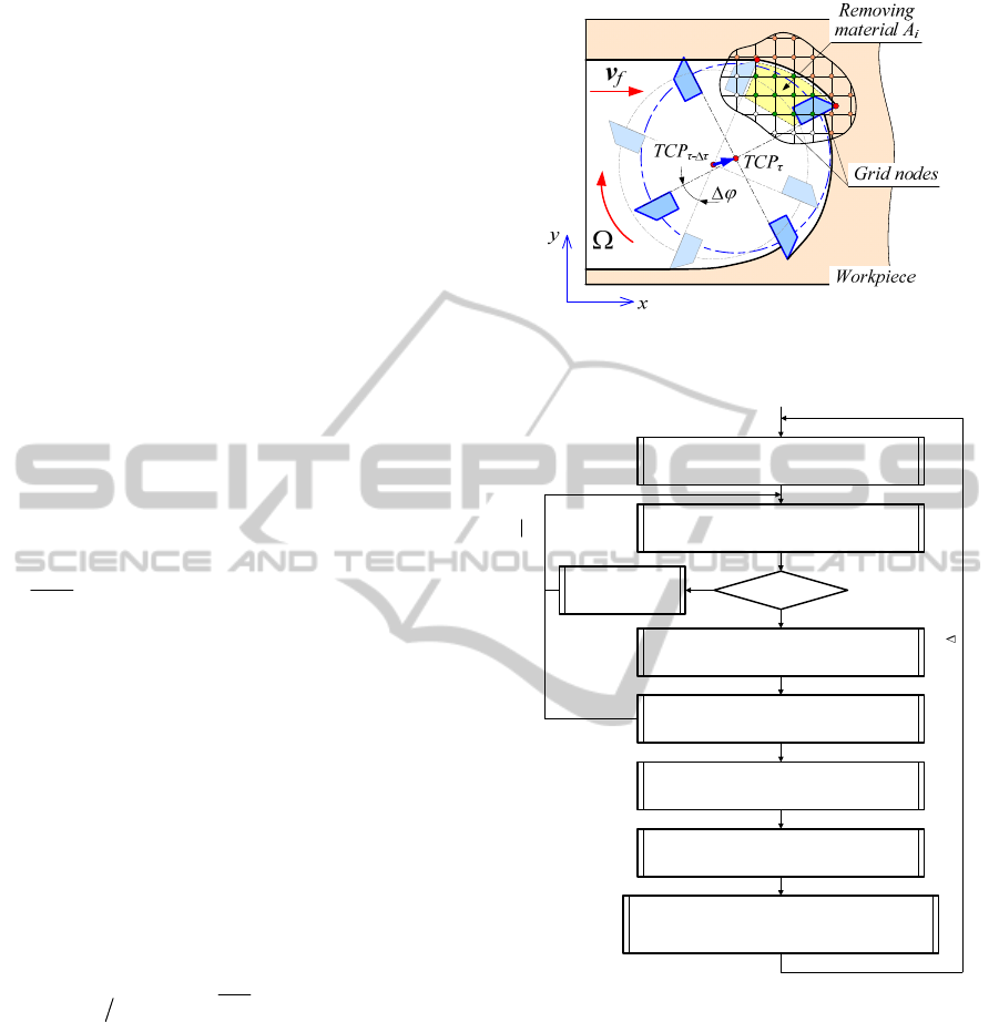
In order to define the number of currently cut
nodes by the
i-th tooth, the previous instant of ma-
chining process should be considered. Let us define
A
i
as an amount of working material that is currently cut
away by the
i-th tooth (Figure 5). So, if node j marked
as “1” is located inside the marked sector (green
nodes in Figure 5), it changes to “0” and
A
i
is increas-
ing by
x
y
s
sΔΔ . Analyzing all potential nodes and
computing
A
i
, the chip thickness h
i
, removed at given
instant of the process by the
i-th tooth, can be estimat-
ed by
,
ii i
hAR
α
=Δ
1,
z
iN=
. The angle Δφ
i
deter-
mines the current angular position of the
i-th tooth
regarding to its position at the instant
τ-Δτ and re-
ferred to the position of TCP at
τ-Δτ.
Described mechanism of chip formation and the
machining force model (18) allow computing the dy-
namic behavior of the robotic machining process
where models of robot inertia and stiffness are dis-
cussed in the section 3 of the paper. The detailed algo-
rithm that is used in numerical analysis is presented in
Figure 6, where the analysis of the robot dynamics is
performed in the tool frame with respect to the dy-
namic displacement of the tool
δt
dyn
fixed on the robot
end-effector around its position on the trajectory..
Figure 5: Evaluating the tool/workpiece intersection A
i
and computing the corresponding chip thickness h
i.
.
Computing the position of TCP and position/
orientation of all teeth (tool frame)
Analysis of interaction between j-th tooth and
grid nodes, computing A
j
Updating the grid, computing the chip
thickness h
j
Definition of the external loading caused by
technological process (tool frame) :
F=[F
x
F
y
0 0 0 0]
T
A
j
>0
Repeat for all teeth
Yes
No
Zero cutting
forces, F
rj
=0, F
tj
=0
Computing the radial and tangential cutting
force components F
rj
, F
tj
Computing the machining forces F
x
, F
y
(tool
frame)
Analysis of dynamics of the robotic machining
process (tool frame)
Next time step τ : τ=τ
0
: τ:τ
MAX
Zj ,1=
11 1
dyn c c dyn c c dyn c
−− −
=− − +δtMCδtMKδtMF
&& &
Figure 6: Algorithm for numerical simulation of robotic
machining process dynamics.
5 COMPLIANCE ERROR
COMPENSATION TECHNIQUE
In industrial robotic controllers, the manipulator mo-
tions are usually generated using the inverse kine-
matic model that allows us to compute the input sig-
nals for actuators
0
ρ corresponding to the desired
end-effector location
0
t , which is assigned assum-
ing that the compliance errors are negligible. How-
ever, if the external loading
F is essential, the kin-
ICINCO2012-9thInternationalConferenceonInformaticsinControl,AutomationandRobotics
118
ematic control becomes non-applicable because of
changes in the end-effector location. It can be com-
puted from the non-linear compliance model as
(
)
1
F0
|f
−
=tFt (22)
where the subscripts 'F' and '0' refer to the loaded
and unloaded modes respectively, and '
| ' separates
arguments and parameters of the function
(
)
f .
Some details concerning this function are given in
our previous publication (Pashkevich, 2011).
To compensate this undeterred end-effector dis-
placement from
0
t to
F
t , the target point should be
modified in such a way that, under the loading
F , the
end-platform is located in the desired point
0
t . This
requirement can be expressed using the stiffness
model in the following way
()
(F)
00
|f=Ftt (23)
where
(F)
0
t denotes the modified target location.
Hence, the problem is reduced to the solution of the
nonlinear equation (23) for
(F)
0
t , while F and
0
t are
assumed to be given. It is worth mentioning that this
equation completely differs from the equation
0
(| )f=Ftt, where the unknown variable is t . It
means that here the compliance model does not al-
low us to compute the modified target point
(F)
0
t
straightforwardly, while the linear compensation
technique directly operates with Cartesian compli-
ance matrix (Gong, 2000).
To solve equation (23) for
(F)
0
t , similar numerical
technique can be applied. It yields the following itera-
tive scheme
(
)
(F) (F) 1 (F)
00 0 0
(| )· f
α
−
=+ −
′
tt t Ft (24)
where the prime corresponds to the next iteration,
(0,1)
α
∈
is the scalar parameter ensuring the con-
vergence. More detailed presentation of the devel-
oped iterative routines is given in Figure 7.
()
Ft
)F(1
0
| εf
−
−<Ftt
()
1(F)
0
|f
−
=
F
tFt
{
}
{
}
0
;()
j
j
∈=∈ttF0FFt
()
{
}
j
j
∈ttFt
{
}
0 j
∈tt
(
)
(F) (F)
00 0
α
=+
′
⋅
−
F
tt tt
0
(F)
0
=
tt
()
C
,,,
iii
i
qFKθ
Figure 7: Procedure for compensation of compliance er-
rors.
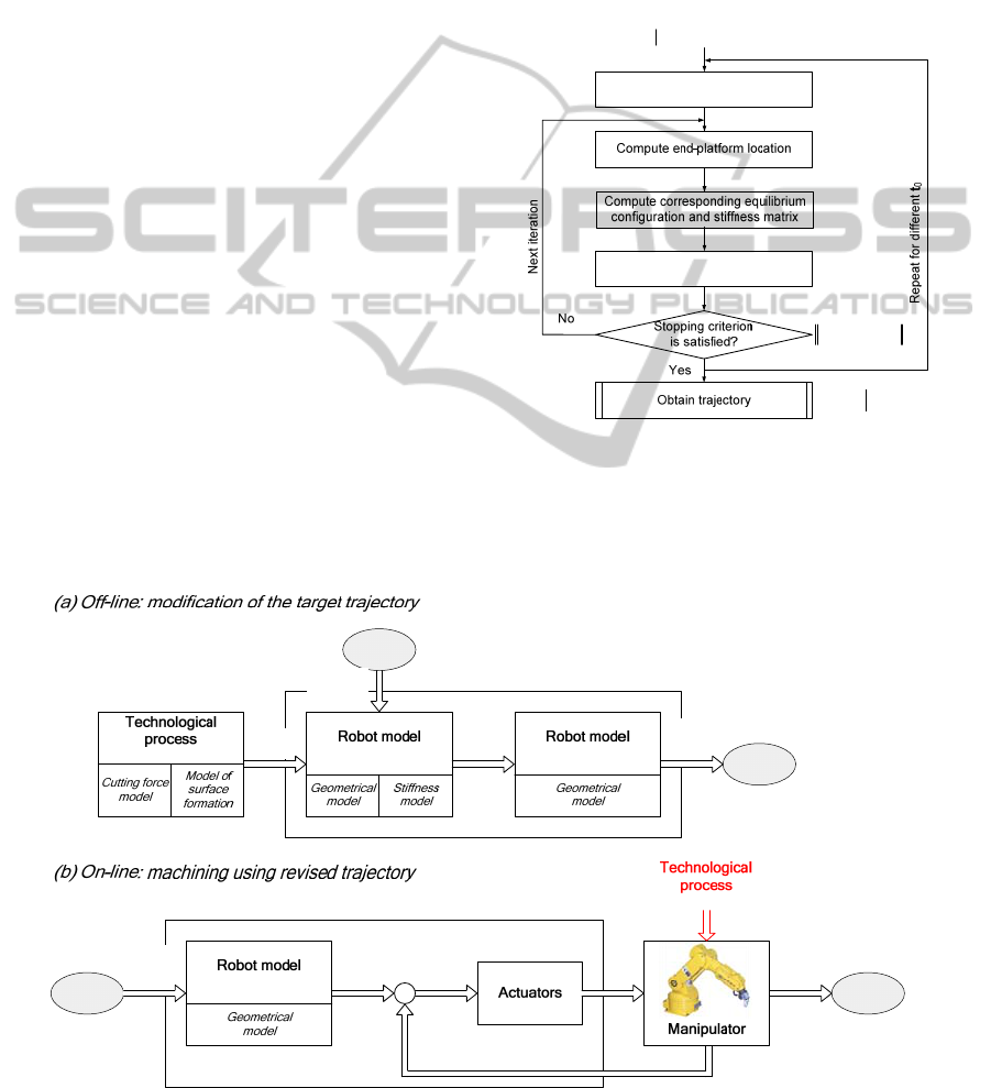
Hence, using the proposed computational tech-
niques, it is possible to compensate a main part
Modified
trajectory
-
Cartesian
coordinates
Joint
encoders
Joint
coordinates
Cartesian
coordinates
Robot Controller
Actual joint coordinates
Obtained
trajectory
(nominal)
direct
(actual)
Estimated
loading
(nominal)
Error compensator
Joint
coordinates
Desired
trajectory
inverse
Cartesian
coordinates
Modified
trajectory
direct
Cartesian
coordinates
(actual)
(actual)
Figure 8: Implementation of compliance error compensation technique.
CompensationofToolDeflectioninRobotic-basedMilling
119
compliance errors by proper adjusting the reference
trajectory that is used as an input for robotic control-
ler. In this case, the control is based on the inverse
kinetostatic model (instead of kinematic one) that
takes into account both the manipulator geometry and
elastic properties of its links and joints. Implementa-
tion of developed compliance error compensation
technique presented in Figure 8.
6 EXPERIMENTAL
VERIFICATION
The developed compliance error compensation tech-
nique has been verified experimentally for robotic
milling with the KUKA KR270 robot along a simple
trajectory in aluminum workpiece. It is assumed that
at the beginning of the technological process the robot
is in the configuration
q (see Table 1 Figure 9). The
parameters of the stiffness model for the considered
robot have been identified in (Dumas, 2011) and are
presented in Table 1. Link masses required for the
mass matrix of the robot are presented also in Table 1.
Table 1: Initial data for robotic-based milling.
Joint coordinates, [deg]
q
1
q
2
q
3
q
4
q
5
q
6
90 -50 120 180 25 180
Joint compliances, [rad/N m]*10
-6
k
1
k
2
k
3
k
4
k
5
k
6
0.26 0.15 0.26 1.79 1.52 2.13
Link masses, [kg]
m
1
m
2
m
3
m
4
m
5
m
6
336.8 259.4 85.2 54.5 36.3 18.2
Figure 9: Starting pose of the KUKA KR270 robot to per-
form the operation of milling.
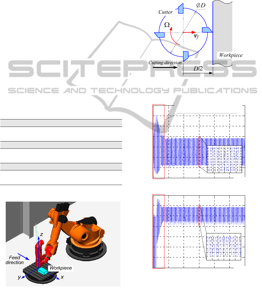
For the milling, the cutter with the external diame-
ter
D=20 mm and four teeth (N
z
=4) distributed uni-
formly over the tool is used. For the given combina-
tion of the tool and the workpiece material the follow-
ing parameters correspond to the cutting force model
defined in (18):
k
0
=
6
510×
N/m, h
s
=
5
1.8 10
−
×
m,
r=0.1, k
r
=0.3.
Figure 10: Starting relative position of the tool with re-
spect to the workpiece.
0 0.2 0.4 0.6 0.8 1 1.2
0
50
100
150
200
250
300
350
0 0.2 0.4 0.6 0.8 1 1.2
-200
-150
-100
-50
0
50
100
150
F
x
,[N] (workpiece→tool)
τ,[s]
Transient phase of tool engagement
into the workpiece (τ
1
=0.15s)
(a)
F
y
,[N] (workpiece→tool)
τ,[s]
(b)
1 1.005 1.01 1.015 1.02 1.025 1.03
-110
-100
-90
-80
-70
-60
-50
-40
-30
-20
-10
1 1.005 1.01 1.015 1.02 1.025 1.03
170
180
190
200
210
220
230
240
Figure 11: Variation of machining force components F
x
(a)
and F
y
(b) for whole milling process.
ICINCO2012-9thInternationalConferenceonInformaticsinControl,AutomationandRobotics
120
Taking into account that the workpiece has a
straight borders let us assume that at the instant t=0
one of the teeth of the tool is in contact with the
workpiece material as it is shown in the Figure 10. It
is also assumed that the machining process is per-
forming with the constant feed rate
v
f
=4 m/min (ap-
plied in
x-direction of the robot tool frame) and the
constant spindle rotation Ω=8000 rpm along the
straight line of 80 mm. Experimental verification and
numerical simulation of the described case of the
milling process with KUKA KR-270 robot using the
algorithm shown in Figure 6 allows us to trace the
evolution of machining force x,y-components for the
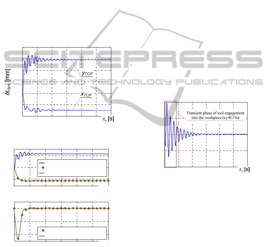
whole process (Figure 11). The corresponding dy-
namic displacement of the tool around its current po-
sition on the trajectory is shown in Figure 12.
0 0.2 0.4 0.6 0.8 1 1.2
-0.04
-0.02
0
0.02
0.04
0.06
0.08
Figure 12: Evolution of the tool dynamic displacement
δt
dyn
that is composed from x
TCP
and y
TCP
components.
0 0.2 0.4 0.6 0.8 1 1.2
-5
0
5
x 10
-
5
0 0.2 0.4 0.6 0.8 1 1.2
-4
-2
0
x 10
-5
f
y
, y
TCP
, [mm]
10
-2
v
fy
, [m/s]
τ,[s]
τ,[s]
y
TCP
Referenced points
Modified trajectory in y-direction
Referenced points
Modified feed rate in y-direction
Figure 13: Modified trajectory f
y
and corresponding feed
rate v
fy
in y-direction, computed based on the original dy-
namic displacement of the tool δt
dyn
.
In accordance with the obtained results the system
robot/machining process realize complex vibratory
motion. The high frequency component of this motion
(about 700 Hz, Figure 11) is related to the spindle ro-
tation and the number of tool teeth
N
z
. In certain cases
such behavior can excites the dynamics of the robot
(natural modes) but this study remains out the frame
of the presented paper. On the contrary, the low fre-
quency component of robot/tool motion (about 7 Hz,
Figure 12), especially in the
y-direction (that is per-
pendicular to the applied feed) influences directly the
quality of final product. Such motion is related to the
robot compliance and it can be compensated using the
error compensation technique described in the paper.
Hence, let us form the modified trajectory based on
the dynamic displacement of the robot end-effector in
the
y-direction (Figure 13):
It should be stressed that the time step between
referenced points of this modified trajectory is limited
with the characteristics of the controller used in the
robot (in the presented case this step is chosen 0.05
sec). The corresponding feed rate
v
fy
for the modified
trajectory has been computed. So, this new data (feed
f
y
and feed rate v
fy
) with the data defined in the begin-
ning of this section allow us to compensate the trajec-
tory error during machining caused by the robot com-
pliance. The resulted compensated trajectory in the y-
direction (in time domain) is presented in Figure 14.
0 0.2 0.4 0.6 0.8 1 1.2
-0.02
-0.01
0
0.01
0.02
y
TCP
after compensation, [mm]
Figure 14: Evolution of the dynamic displacement ob-
tained after involving the error compensation technique
into the analysis of robotic milling process.
It should be noted that the part of the trajectory
while machining tool is engaging into the workpiece
does not have effect on the quality of final product (sur-
face). During this stage the contact area between the
tool and the workpiece is increasing progressively.
Hence, at each instant of processing the cutter corrects
the machining profile and eliminates trajectory errors
produced during all previous instants. On the contrary,
during the stage of machining with the fully engaged
tool the trajectory in x,y-directions define directly the
final machining profile and this part of trajectory is
analyzed here (Figure 14). Comparison results present-
ed in Figure 12 and Figure 14 are summarized in Table
2. So after applying error compensation technique the
static deviation in y direction has been reduced from
CompensationofToolDeflectioninRobotic-basedMilling
121

0.058 mm to 0.00014 mm (99.8%). Maximum
defilation in the machining profile has been reduced
from 0.063 mm to 0.0047 mm (92.6%). Low frequency
remained the same for both cases.
Table 2: Milling trajectory accuracy before and after com-
pliance error compensation.
Performance measure
Original
trajectory
Modified
trajectory
Low frequency,[ Hz] 6.70 6.70
Static deviation y
s
, [mm] 58.1e-3 0.14e-3
Max deviation y
MAX
,
[mm]
63.2e-3 4.70e-3
Hence, obtained results show that the developed com-
pliance error compensation allows us significantly
increase the accuracy of the robotic-based machining.
7 CONCLUSIONS
In robotic-based machining, an interaction between
the workpiece and technological tool causes essential
deflections that significantly decrease the manufactur-
ing accuracy. Relevant compliance errors highly de-
pend on the manipulator configuration and essentially
differ throughout the workspace. Their influence is
especially important for heavy serial robots. To over-
come this difficulty this paper presents a new tech-
nique for compensation of the compliance errors
caused by technological process. In contrast to previ-
ous works, this technique is based on the non-linear
stiffness model and the reduced elasto-dynamic model
of the robotic based milling process.
The advantages and practical significance of the
proposed approach are illustrated by milling with of
KUKA KR270. It is shown that after error compensa-
tion technique significantly increase the accuracy of
milling. In future the proposed technique will be inte-
grated in a software toolbox.
ACKNOWLEDGEMENTS
The authors would like to acknowledge the financial
support of the ANR, France (Project ANR-2010-
SEGI-003-02-COROUSSO) and the Region “Pays de
la Loire”, France.
REFERENCES
Alici G., Shirinzadeh B., 2005. Enhanced stiffness model
ing, identification and characterization for robot manip-
ulators. Proceedings of IEEE Transactions on Robotics,
vol. 21, pp. 554–564.
Altintas Y., 2000. Manufacturing automation, metal cutting
mechanics, machine tool vibrations and CNC design.
Cambridge University Press, New York.
Brissaud D., Gouskov A., Paris H., Tichkiewitch S., 2008.
The Fractional Model for the Determination of the Cut-
ting Forces. Asian Int. J. of Science and Technology -
Production and Manufacturing, vol. 1, pp.17-25.
Briot S., Pashkevich A., Chablat D. Reduced elastodynamic
modelling of parallel robots for the computation of their
natural frequencies. 13th World Congress in Mechanism
and Machine Science, 19 - 25 Juin, 2011, Guanajuato,
Mexico.
Chen S., Kao I., 2000. Conservative Congruence Transfor-
mation for Joint and Cartesian Stiffness Matrices of Ro-
botic Hands and Fingers. The International Journal of
Robotics Research, vol. 19(9), pp. 835–847.
Dépincé P., Hascoët J-Y., 2006. Active integration of tool
deflection effects in end milling. Part 2. Compensation
of tool deflection, International Journal of Machine
Tools and Manufacture, vol. 46, pp. 945-956
Dumas C., Caro S., Garnier S., Furet B., 2011. Joint stiff-
ness identification of six-revolute industrial serial ro-
bots, Robotics and Computer-Integrated Manufactur-
ing, vol. 27(4), pp. 881-888.
Eastwood S. J., Webb P., 2010. A gravitational deflection
compensation strategy for HPKMs, Robotics and Com-
puter-Integrated Manufacturing, vol. 26 pp. 694–702
Gong, C., Yuan J., Ni, J., 2000. Nongeometric error identi-
fication and compensation for robotic system by inverse
calibration. International Journal of Machine Tools &
Manufacture, vol. 40(14) pp. 2119–2137.
Kövecses J., Angeles J., 2007. The stiffness matrix in elas-
tically articulated rigid-body systems. Multibody System
Dynamics. vol. 18(2), pp. 169–184.
Laporte S., K’nevez J.-Y., Cahuc O., Darnis P., 2009. Phe-
nomenological model for drilling operation. Int. J. of
Advanced Manufacturing Technology, vol.40, pp.1-11.
Merchant M. E., 1945. Mechanics of metal cutting process.
I-Orthogonal cutting and type 2 chip. Journal of Applied
Physics, vol.16(5), pp.267–275.
Pashkevich A., Klimchik A., Chablat D., 2011. Enhanced
stiffness modeling of manipulators with passive joints.
Mech. and Machine Theory, vol. 46(5), pp. 662-679.
Ritou M., Garnier S., Furet B., Hascoet J.Y., 2006. A new
versatile in-process monitoring system for milling, Int.
J. of Machine Tools & Manufacture, 46/15:2026-2035.
Tlusty J., Ismail F., 1981, Basic non-linearity in machining
chatter. Annals of CIRP, Vol.30/1, pp.299-304.
Tyapin I., Hovland G., 2009. Kinematic and elastostatic de-
sign optimization of the 3-DOF Gantry-Tau parallel
kinamatic manipulator. Modelling, Identification and
Control, vol. 30(2), pp. 39-56
Su H.-J., McCarthy J. M., 2006. A Polynomial Homotopy
Formulation of the Inverse Static Analyses of Planar
Compliant Mechanisms. Journal of Mechanical Design
,
vol. 128(4), pp. 776-786.
ICINCO2012-9thInternationalConferenceonInformaticsinControl,AutomationandRobotics
122
