A Bug-based Path Planner Guided with Homotopy Classes

Emili Hern

andez, Marc Carreras and Pere Ridao

Department of Computer Engineering, University of Girona, 17071 Girona, Spain

Keywords:

Path Planning, Homotopy Classes, Robotics.

Abstract:

This paper proposes a bug-based path planning algorithm guided topologically with homotopy classes. Ho-

motopy classes provide a topological description of how paths avoid obstacles in the workspace. They are

generated with a method we developed, which builds a topological environment based on the workspace that

allows to compute homotopy classes systematically. The homotopy classes are sorted according to a heuristic

estimation of their lower bound. Only those with the smaller lower bound are used to guide the path planner we

propose, called Homotopic Bug (HBug), which efﬁciently computes paths in the workspace that accomplish

homotopy classes. Results show the feasibility of our method. A comparison with well-known path planners

has also been included.

1 INTRODUCTION

The work presented in this paper is focused on the

design of a navigation system for a robot that is able

to detect the environment, build an internal local map

of the explored area according to the information pro-

vided by the onboard sensors, compute a safe path

through the map and, ﬁnally, generate the high-level

commands to follow it. The navigation system has to

be able to generate an Occupancy Grid Map (OGM)

and a path according to the information obtained from

the unknown environment in a reduced amount of

time. The target application of this research project

is autonomous navigation for surveilling and explo-

ration tasks in unstructured environments.

Given an OGM, this paper addresses the design of

a path planning algorithm to generate a path in a very

short time. Anytime path planners (Ferguson et al.,

2005) have been shown suitable to be used with robots

that have a limited amount of time to perform path

planning. These algorithms compute an initial solu-

tion highly suboptimal very fast and improves it un-

til time runs out. Deterministic anytime approaches,

like the Anytime Repairing A* (ARA*) (Likhachev

et al., 2004), speed up the path generation by inﬂating

the heuristics to force the exploration of those conﬁg-

uration that are closer to the goal according to their

heuristics. During successive iterations the inﬂation

factor is decreased in order to generate improved so-

lutions. On the other side, sampling-based anytime

algorithms such as Anytime-RRT (ARRT) (Ferguson

and Stentz, 2006), generate a series of RRTs where

each new tree reuses the cost information from the

previous tree to control its growth and thus improve

the quality of the resultant path. At each iteration,

anytime path planners try to improve the solution by

decreasing the heuristics/cost inﬂation. However, the

generation of a new/better path is not ensured (a path

with the same cost can be obtained).

Topological approaches are another way to tackle

the path planning problem. This kind of solu-

tions work with a graph-based abstraction of the

workspace, in which the environment is represented

by a reduced number of potential states over the afore-

mentioned strategies (Dudek et al., 1991; Fabrizi and

Safﬁotti, 2000). Visibility graphs (Latombe, 1991)

and voronoi diagrams (Takahashi and Schilling,

1989) constitute well-known approaches in this re-

gard. Other methods use homotopy classes to provide

a topological description of how paths avoid obsta-

cles. Two paths that share the start point and the end

point belong to the same homotopy class if one can be

deformed into the other without encroaching any ob-

stacle. Some authors compute the shortest homotopic

path of a given input path (Chazelle, 1982; Grigoriev

and Slissenko, 1998; Efrat et al., 2002; Bespamyat-

nikh, 2003). However, in most of robotics applica-

tions the path is not known in advance. (Fujita et al.,

2003; Bhattacharya et al., 2010) generate an initial

path, whose homotopy class is then obtained in order

to prevent the algorithm to generate another path with

the same topology. This methodology achieves the

123

Hernández E., Carreras M. and Ridao P..

A Bug-based Path Planner Guided with Homotopy Classes.

DOI: 10.5220/0004041201230131

In Proceedings of the 9th International Conference on Informatics in Control, Automation and Robotics (ICINCO-2012), pages 123-131

ISBN: 978-989-8565-22-8

 2012 SCITEPRESS (Science and Technology Publications, Lda.)

generation of a path for different homotopy classes by

blocking those previously explored, which make them

suitable for computing the shortest path, but not for

generating a solution with a different homotopy, since

it would require to compute several paths to achieve

the desired solution. To overcome this problem, some

methods (Jenkins, 1991; Schmitzberger et al., 2002)

ﬁrst generate a set of homotopy classes, allowing to

look directly for a path with a speciﬁc topology. How-

ever, they require establishing a set of restriction cri-

teria in order to generate only those homotopy classes

that have an interest for the problem we need to solve.

A solution to this problem has been has been proposed

in (Hern

andez et al., 2011a; Hern

andez et al., 2011c).

In this paper we propose a bug-based path planner

called Homotopic Bug (HBug), which is guided topo-

logically with homotopy classes. Although bug al-

gorithms were initially conceived to achieve reactive

online navigation for robots with low computational

capabilities in unknown scenarios, it is also possible

to use them to perform deliberative path planning on

a Conﬁguration Space (C-space) (Antich et al., 2009).

The HBug follows the homotopy classes generated

with a method we presented in (Hern

andez et al.,

2011a) and improved in (Hern

andez et al., 2011c).

Using the topological information, the path planner

does not have to explore the whole space but the

space conﬁned in a homotopy class, speeding up the

path computation. Moreover, homotopy classes allow

the generation of paths that avoid obstacles in differ-

ent manners, which is interesting for surveilling pur-

poses. Unlike anytime approaches, which start the

path search with a highly suboptimal solution, the

HBug starts looking for a path in a homotopy class

that has a high probability of containing the optimal

solution. The method is proved to be complete be-

cause in case the goal is not reachable, no homotopy

classes will exist and, consequently, no paths will be

generated. It is important to note that the homotopy

class of the global optimal path is guaranteed to be

generated by the algorithm. Results and comparison

with other path planners show the efﬁciency and the

performance of our method, achieving near to opti-

mal solutions with respect to the homotopy class in

unstructured environments with irregular obstacles,

which are the target scenarios of our method.

The paper is structured as follows. Section 2

summarizes the method to generate homotopy classes

from the workspace. Section 3 describes the

topologically-guided path planning algorithm that we

propose. Section 4 reports the results, and section 5

exposes the conclusions and future work.

2 HOMOTOPY CLASSES OF THE

WORKSPACE

Two paths that share the start point and the end point

belong to the same homotopy class if one can be de-

formed into the other without encroaching any obsta-

cle. Therefore, homotopy classes provide topological

information of how paths that belong to a class would

avoid the obstacles. In (Hern

andez et al., 2011c)

we presented a method to compute all the homotopy

classes of any 2D workspace, whose steps are sum-

marized in the following sections.

2.1 Reference Frame

The reference frame determines in the metric space

the topological relationships between obstacles and it

is used to name the homotopy classes. To build it, ev-

ery obstacle is represented by a single point b

. Then,

a set of lines join each b

point and a cental point c

placed in the free space. The lines are partitioned into

segments according the intersections with the obsta-

cles and labeled α

or β

depending on the side of

the obstacle they rely on, where k is the obstacle in-

dex and s is the segment index within the line.

The reference frame allows to represent any path

as the sequence of labels of the segments being

crossed in order from the starting to the ending point.

For instance, Figure 1a depicts a reference frame

for a scenario with two obstacles. The path that

traverses it is labeled β

−1

Notice that this path is topologically equivalent to

−1

, which is the canonical sequence of

the homotopy class, since is the simplest repre-

sentation of a path without changing its topology

(Hern

andez et al., 2011c).

2.2 Topological Graph

The topological graph, whose construction is based

on the reference frame, provides a model to de-

scribe the topological relationships between regions

of the metric space. The reference frame divides the

workspace into several regions. Each region repre-

sents a node of the topological graph. The nodes are

interconnected according to the number of segments

they share in the reference frame. Each edge of the

graph is labeled with the same label of the segment

that crosses in the reference frame.

In the reference frame, a path is deﬁned according

to the segments it crosses whereas in the topological

graph it turns into traversing the graph from the start-

ICINCO2012-9thInternationalConferenceonInformaticsinControl,AutomationandRobotics

124

−

3.2

3.1

−

1.1

4.1 2.1

−

1.2

a) Reference frame b) Topological graph

Figure 1: Topological path represented in the reference

frame as p = β

−1

and its canoni-

cal sequence (β

−1

) in the topological graph.

ing node to the ending node

. Figure 1a depicts a path

in the reference frame and Figure 1b its equivalent de-

scription in the topological graph.

2.3 Generation of Homotopy Classes

Once the topological graph is constructed, it is tra-

versed with a modiﬁed version of the Breadth-First

Search (BFS) algorithm used in (Hern

andez et al.,

2011a; Hern

andez et al., 2011c), which incrementally

builds the candidate homotopy classes according to

the edges traversed during the graph search. The al-

gorithm stops when there are no more homotopy class

candidates to explore or the length of the last homo-

topy class candidate is larger than a given threshold.

Notice that those homotopy classes which either self-

intersect or whose canonical sequence is duplicated

are not considered (Hern

andez et al., 2011b).

2.4 Lower Bound

Depending on the number of homotopy classes gener-

ated by the BFS algorithm, it is not possible to com-

pute all their correspondent paths in the workspace in

real-time. Therefore, we have modiﬁed the funnel al-

gorithm (Chazelle, 1982) to obtain a quantitative mea-

sure for each homotopy class estimating their quality.

This algorithm computes the shortest path within a

channel, which is a polygon formed by the vertexes of

the segments of the reference frame that are traversed

in the topological graph. The modiﬁcation consists

of accumulating the Euclidean distance between the

points while they are being added to the shortest path.

Hence, the result of the funnel algorithm is a lower

bound of the optimal path in the workspace of the se-

lected homotopy class, which is used to set up a pref-

Starting and ending nodes are those regions in the refer-

ence frame where the starting and ending points are located.

linem

−

Figure 2: Example of execution of Bug2 algorithm in a sim-

ple scenario.

erence order to compute the homotopy classes path in

the workspace. Figure 3a depicts an example where

the funnel algorithm computes the lower bound for

the homotopy class β

−1

. The solid lines

represents the channel and the dashed line is the path

after applying the algorithm. Notice that our vari-

ant of the funnel algorithm takes into account that

some subsegments may self-intersect when creating

the channel (α

and α

in Figure 3a).

3 BUG-BASED PATH PLANNING

Once the homotopy classes are computed and sorted

according to their lower bound, a path planning algo-

rithm has to ﬁnd a path in the workspace that follows a

given homotopy class, which essentially implies turn-

ing a topological path into a metric path. The only

link between the workspace and the topological space

is the reference frame. It allows checking whether

a metric path in the workspace is following a topo-

logical path by following the intersections –in order–

from the initial conﬁguration to the current conﬁgura-

tion.

3.1 The Bug2 Algorithm

Our proposal is a path planning algorithm based on

the Bug2 (Lumelsky and Stepanov, 1987). The Bug2

starts by setting up an imaginary line, called m-line,

which connects the start point with the goal point. The

robot starts by following the m-line until the contact

point with an obstacle, which is the ﬁrst hit point h

Then, a boundary following behavior surrounds the

obstacle until it reaches a point in the m-line which is

closer to the goal than the previous hit point, that is

the ﬁrst leave point l

. The same process is repeated

until the goal is found. Figure 2 depicts a path gen-

erated by the Bug2 algorithm. Note that the direction

to circumnavigate the obstacles can be ﬁxed at the be-

ginning of the execution or chosen randomly.

ABug-basedPathPlannerGuidedwithHomotopyClasses

125

3.2 Homotopic Bug

As stated before, the path planning algorithm we pro-

pose, which is called Homotopic Bug (HBug), is

based on the Bug2. Essentially, it tries to follow di-

rectly the lower bound path obtained with the mod-

iﬁed funnel algorithm, which ensures that the ho-

motopy class is being accomplished. However, the

segments of the reference frame constrain the region

where the paths can go through, but do not take into

account the shape of the obstacles. For this reason, the

lower bound path may intersect with the obstacles. In

such case, the obstacle boundary is followed in clock-

wise or counterclockwise direction according to the

homotopy class until the lower bound path leaves the

obstacle. This process is repeated for all the inter-

sected obstacles by the lower bound path.

The HBug, detailed in Algorithm 1, receives as

an input parameters the lower bound path P, a can-

didate homotopy class to follow H and the reference

frame F. Notice that the ﬁrst and the last elements of

P are the start (s) and goal (g) nodes respectively. The

algorithm is a three step process. First, the function

BoundaryNodes checks the intersections of P with

the obstacles in the C-space. Every time that P hits or

leaves an obstacle, a boundary node is created. Each

node contains the contact point c and the obstacle la-

bel k, which is the subindex of the point b

that rep-

resents the obstacle in the reference frame. These pa-

rameters are accessible through the functions Q and

Obst respectively. Then, ObstacleNodes computes

the nodes O based on the boundary nodes N previ-

ously computed. Each obstacle node contains the ﬁrst

boundary node that hits the obstacle n

, the last node

that is in its boundary without changing the obstacle

, and the direction d to surround the obstacle while

following H (line 23). Finally, the function BuildPath

creates the path P

in the workspace by joining the

boundary of each obstacle o

∈ O from n

to n

with

the direction d.

The direction d to surround an obstacle is set ac-

cording to the direction of a hit node n

towards its

successor n

h+1

respect to the point b

, that represents

the obstacle of the workspace in the reference frame.

Notice that n

and n

h+1

are ensured to belong to the

same obstacle since for any point that hits an obstacle

there has to be another one that releases it. The per-

pendicular dot product between vectors (Q(n

) − b

)

and (Q(n

h+1

)−b

) computes the boundary following

direction (line 15). If the result is less than 0 the di-

rection from n

to n

h+1

is counterclockwise; if it is

greater than 0 the direction is clockwise.

When the lower bound path intersect with obstacle just

one time, the n

h+1

node is also the n

node.

Algorithm 1: Homotopic Bug.

BoundaryNodes(P)

1: N ←

2: for i ← 1 to |P| − 1, p

∈ P do

3: C ← ContourPoints(p

, p

i+1

)

4: for all j ← 1 to |C|,c

∈ C do

5: k ← Label(c

)

6: N ← N ∪ {c

,k}

7: end for

8: end for

9: return N

ObstacleNodes(N, H, F)

10: O ←

11: h ← 1

12: while n

∈ N/h < |N| − 1 do

13: n

← last n

∈ N/ j > h without changing Obst(n

)

14: b

← point of Obst(n

) in F

15: d ← (Q(n

) − b

)

⊥

· (Q(n

h+1

) − b

)

16: if d = 0 then {parallel}

17: d ← (s − b

)

⊥

· (point of 1

∈ H −b

)

18: i

← index of χ

∈ H where n

h+1

relies on

19: if |χ

| ∈ H

1..i

is even then

20: switch d

21: end if

22: end if

23: O ← O ∪ {n

,d}

24: h ← l + 1

25: end while

26: return O

BuildPath(O)

27: P

←

28: for i ← 1 to |O|,o

∈ O do

29: P

← P

∪ Boundary(o

)

30: end for

31: return P

HBug(P,H, F)

32: N ← BoundaryNodes(P)

33: O ← ObstacleNodes(N, H, F)

34: P

← BuildPath(O)

The result of the perpendicular dot product can

be 0 if the vectors (Q(n

) − b

) and (Q(n

h+1

) − b

)

are parallel, which means that n

, n

h+1

and b

be-

long to the same l

in the reference frame (line 16).

In such case, d is obtained according two conditions:

the initial direction selected to cross l

from the start

point, and the number of times that l

is crossed until

the α

or β

–denoted by χ

– of the homotopy class,

where n

h+1

relies on, is reached. The initial direction

is obtained with the dot product form the start s to

the ﬁrst χ

with the same subindex than l

(line 17).

The number of times that l

is crossed depends on the

number of χ

found in the homotopy class from the

beginning to the index i

, which indicates the position

Notice that the start point cannot be in a line l

of the

reference frame since the perpendicular dot product would

be also 0.

ICINCO2012-9thInternationalConferenceonInformaticsinControl,AutomationandRobotics

126

−

}2,{:

ccw

}2,{:

}

{

}1,{:

−

}

{

a) Channel and lower bound path b) Path computed with the HBug

Figure 3: Generation of the lower bound path and the HBug

path for the homotopy class β

−1

of the χ

that contains n

h+1

(line 19).

Figure 3 depicts an example scenario where the

HBug is applied. The homotopy class to follow is

−1

. The dashed line represents its lower

bound path, which intersects with the ﬁrst obstacle

generating two boundary nodes n

and n

, both of

them located on the line l

of the reference frame.

The point that represents the obstacle is b

, also on

, which makes perpendicular dot product between

(Q(n

) − b

) and (Q(n

) − b

) unable to set the di-

rection (d = 0). Therefore, using the start point s

and a point of the edge β

, the initial direction is set

clockwise (cw). The last edge involved in this situ-

ation is α

, which is located in the second position

in the homotopy class. The number of edges with

subindex 1 till this position is 2. Thus, the direction

is not changed. Then, the lower bound path intersects

with the second obstacle in n

and n

. Using the base

point b

, the perpendicular dot product sets the direc-

tion as counterclockwise (ccw). Finally, the path is

composed from s to g with the boundaries of the ob-

stacle 1 (from n

to n

) and the obstacle 2 (from n

) joint by straight lines.

4 RESULTS

The feasibility the topological path search with the

HBug has been tested in different bitmap scenarios

which have been used as C-spaces, where the robot is

represented as a single point. To identify the obsta-

cles of the scenarios we have adapted a Component-

Labeling (CL) algorithm that efﬁciently labels con-

nected cells and their contours in greyscale images

at the same time (Chang et al., 2004). The contours

of the obstacles provided by this algorithm are used

by the HBug to avoid recomputing them at each new

path search. For the construction of the reference

frame, the c point has been set at a ﬁxed position in

2-α

8-β

3-α

9-β

Figure 4: Paths for the four homotopy classes with the

smaller lower bound in Table 1.

order to ensure the same topological graph construc-

tion –and homotopy classes generation– through dif-

ferent executions. The homotopy classes have been

set at a maximum of 20 characters length. In order

to show all the possible results, no time restrictions

have been taken into consideration. The computations

have been carried out with a laptop equipped with an

Intelr Core

Duo@1.83GHz processor and 2GB of

RAM.

4.1 Cluttered Environment

Our method has been applied in a cluttered environ-

ment using a 200x200 pixels bitmap. Figure 4 de-

picts the scenario with the paths of the best homo-

topy classes, according to their lower bound. The

construction of the reference frame, the topological

graph and the generation of the homotopy classes with

their lower bound computation took 7.9ms. Table 1

shows the homotopy classes sorted by their lower

bound with the path cost and the accumulated com-

putation time, which takes into account the homotopy

classes computation and the path generation. The

lower bound and the path cost have been normalized

with the cost of the optimal path computed with the

A* algorithm. It can be appreciated that using the

HBug the computation time for the paths of the 13 ho-

motopy classes is almost negligible (0.374ms) com-

pared with the 7.9ms that takes the rest of the process.

When operating under time restrictions, it is pos-

sible to stop the path search when the lower bound

ABug-basedPathPlannerGuidedwithHomotopyClasses

127

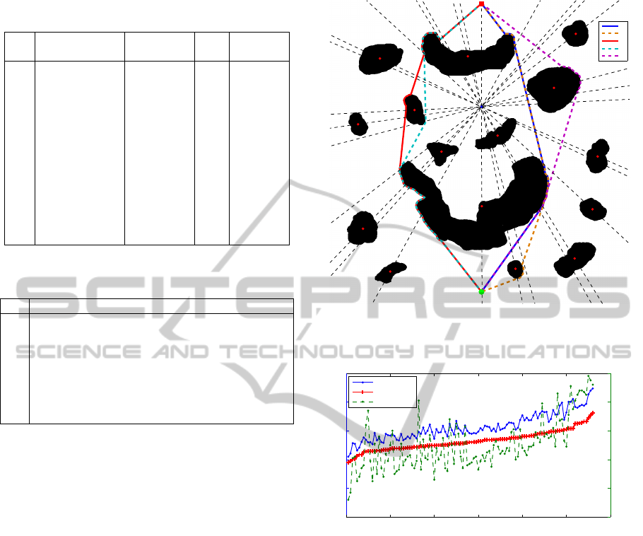
Table 1: Homotopy classes of Figure 4 environment sorted

by their lower bound.

Idx Homotopy class Lower bound Cost Cumulated

time (ms)

2 α

0.93 1.16 7.927

8 β

0.94 1.20 7.950

3 α

0.99 1.43 7.981

9 β

1.00 1.45 8.007

1 α

1.04 1.48 8.035

11 β

1.08 1.53 8.063

10 β

1.13 1.51 8.084

13 β

1.18 1.31 8.106

5 α

1.26 2.02 8.142

4 α

1.32 1.99 8.174

7 α

1.36 1.80 8.205

12 β

1.40 1.77 8.236

6 α

1.58 2.26 8.274

Table 2: The ﬁve homotopy classes of the large environment

with the smaller lower bound and their generation index.

Idx Homotopy class

25 α

−1

−2

26 α

−1

−2

5 α

−1

−2

...

...β

1 α

−1

−2

...

...β

41 α

−1

−2

...

...α

of the next homotopy class –whose path is going to

be computed– is higher than the minimum cost of the

paths already computed. In such case, it is ensured

that the best path with the HBug has been already

computed because it is not possible to obtain a path

with a lower cost than the lower bound. For instance,

in Table 1 the HBug would stop before computing

path for homotopy class with index 13 since its lower

bound (1.18) is higher than the path length obtained

with index 2 class (1.16).

4.2 Scalability

The scalability of the method has been tested in a

bitmap of 1000x1000 pixels with 15 irregular obsta-

cles (Figure 5). The construction of the reference

frame, the topological graph and the generation of

112 homotopy classes with their lower bound compu-

tation took 0.304s. The HBug has been used to com-

pute the path for all homotopy classes of the scenario.

The homotopy classes with the smaller lower bound,

shown in Table 2, and their paths computed with the

HBug are depicted in Figure 5. Figure 6 shows the

cost and computation time for each homotopy class

path computed with the HBug. The homotopy classes

have been sorted according to their lower bound. The

path cost and the lower bound have been normalized

−1

−2

−1

−2

−1

−2

−1

Figure 5: Paths of the ﬁve homotopy classes with the

smaller lower bound computed with the HBug. The class

associated to the index can be found in Table 2.

0 20 40 60 80 100 120

0.5

1.5

2.5

Nº of homotopy class

Lower bound & Cost

0 20 40 60 80 100 120

1.2

1.4

1.6

1.8

x 10

−4

Time (s)

Cost

Lower bound

Time

Figure 6: Normalized cost, normalized lower bound and

computation time for paths generated with the HBug for

each homotopy class.

with respect to the A* path cost. If time restrictions

were applied, the HBug would compute only till the

fourth path.

The fastest path was generated in 1.12x10

−4

s. It

corresponds to the ﬁrst class (index 25) with a path

cost only 1.05 times the optimal solution. The homo-

topy class 110 (index 102) was the one that took more

time to be computed (1.98x10

−4

s) with a cost 2.24

times the global optimal solution. The mean com-

putation per path was only (1.50x10

−4

s). In this en-

vironment, the paths for the whole set of homotopy

classes were computed in 16.8ms, which is almost

negligible when compared with the 304ms spent in the

generation of the reference frame, topological graph

and the generation of the homotopy classes with their

lower bound.

ICINCO2012-9thInternationalConferenceonInformaticsinControl,AutomationandRobotics

128

1.8

RRT

1.4

1.6

1.8

Cost

RRT

Bug2

ARA*

ARRT

HA*

HRRT

1.2

1.4

Cost

HRRT

HBug

0 10 20 30 40 50 60 70 80

Time (s)

1.2

1.3

1.6

1.7

1.8

0.3042

0.3044

0.3046

1.1

0.35

0.4

0.45

0.5

0.55

0.6

1.4

1.5

1.6

0.3042

0.3044

0.3046

0.35

0.4

0.45

0.5

0.55

0.6

Figure 7: Comparison of the HA*, HRRT and HBug paths

of the ﬁve homotopy classes with the smaller lower bound

vs A*, RRT, ARA*, ARRT and Bug2 algorithms.

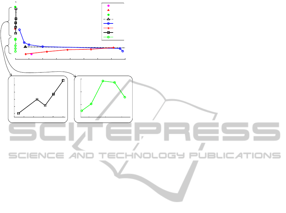
4.3 Path Planners Comparison

The HBug has been compared against the A*, the

RRT, their respective anytime versions (ARA* and

ARRT) and the Bug2 algorithm. The comparison

also includes the results obtained with the Homotopic

A* (HA*) (Hern

andez et al., 2011b) and the Homo-

topic RRT (HRRT) (Hern

andez et al., 2011a), two

path planners that constrain the path search according

to the homotopy classes previously generated. The

A*, the RRT and the Bug2 algorithms are designed

to compute only one path towards the goal; ARA*

and ARRT compute several paths but without tak-

ing into account their homotopy. Because of that,

the comparison with these well-known path planners

are against the ﬁve homotopy classes with the smaller

lower bound (see Table 2). Figure 7 depicts the com-

parison. In order to ensure the stabilization of the re-

sults of the probabilistic path planners, the data ob-

tained with the RRT and the ARRT are the average of

100 executions. Notice that all the time values of the

HA*, HRRT and HBug include the computation time

of the reference frame and topological graph con-

struction, and the generation of the homotopy classes

with their lower bound.

The A* returned the optimal path in 11.90s. The

ARA* generated the ﬁrst solution in 7.40s and found

the optimal solution after 301s. The RRT algorithm

took 0.012s to compute a path with a cost 1.48 times

the global optimal solution. The ARRT took 3.13s

to obtain the ﬁrst solution and 78.30s to compute all

of them, ensuring that any new generated solution is

closer to the optimal one. The Bug2 algorithm com-

puted the path in 0.044s with a cost 1.90 times the

optimal solution. In order to obtain the best possible

path with this algorithm, we have chosen manually

the directions to surround the obstacles: the m-line,

which connects the start with the goal, intersects with

the obstacles labeled b

, b

and b

; the directions are

clockwise for b

, counter-clockwise for b

and clock-

wise for b

The HA* computed the optimal path (index 25) in

7.79s and obtained the path for the ﬁve selected ho-

motopy classes in 71.61s. The HRRT, the best solu-

tion (index 25) was computed in 0.373s with a cost

1.40 times the optimal one, and obtained the path

for the ﬁve homotopy classes with the smaller lower

bound in 0.603s. Using the HBug, our path plan-

ning method computed the best solution (index 25) in

0.304s with a cost 1.05 times the optimal one, and ob-

tained the path for the whole set of homotopy classes

in 0.321s. The computation of the paths with the

HBug for each homotopy class offers a very good per-

formance. Only the RRT and Bug2 had lower com-

putation times at expenses of ﬁnding higher cost so-

lutions. Notice that most of the time was spent in

the computation of the reference frame, the topologi-

cal graph and the generation of the homotopy classes

with their lower bound. The HBug shows a very good

performance because part of its solution is implicitly

generated on the lower bound computation. When

the lower bound path intersects with an obstacle of

the scenario, its boundary is followed in clockwise

or counterclockwise direction according to the homo-

topy class until the lower bound path leaves the obsta-

cle. Notice that the whole boundary of each obstacle

is already computed by the CL algorithm.

The HA* computes the shortest path for each ho-

motopy class, which is the optimal solution according

to the topological constraints. Because of that, Fig-

ure 8 depicts a comparison of the solutions generated

with the HRRT and the HBug against the HA* cost

for each speciﬁc homotopy class. The HRRT gener-

ates solutions between 1.35 (class 15, index 73) and

1.82 (class 83, index 61), with a mean of 1.57 times

with respect the optimal path cost for the speciﬁc ho-

motopy class generated with the HA*. Finally, the

HBug generates solutions between 1.03 (class 5, in-

dex 41) and 1.19 (class 100, index 101), with a mean

of 1.1 times with respect the optimal path cost com-

puted with the HA*.

5 CONCLUSIONS

This paper proposes the HBug path planning algo-

rithm to compute efﬁciently paths that accomplish ho-

ABug-basedPathPlannerGuidedwithHomotopyClasses

129

0 20 40 60 80 100 120

0.9

1.1

1.2

1.3

1.4

1.5

1.6

1.7

1.8

1.9

Nº of homotopy class

Cost

HRRT

HBug

Figure 8: HRRT and HBug paths cost with respect to the

HA* cost for each homotopy class.

motopy classes in any 2D workspace. Given a map

with obstacles, we use a method we developed to gen-

erate systematically the homotopy classes of the en-

vironment. After sorting them according to a lower

bound, the HBug algorithm generates paths in the

C-space following the homotopy classes previously

found. The path planner offers very good perfor-

mance since the path search for a homotopy class

is guided by its lower bound, making the path plan-

ning computation time almost negligible when com-

pared with the time used to generate the homotopy

classes. Results obtained with the HBug, have shown

up that it is a homotopic path planner suitable for

robots with very limited computational capabilities or

applications in which the time to perform path plan-

ning is highly constrained.

Future work will consists in applying our method

into one of the vehicles of our lab. The HBug will be

improved by taking into account the robot’s kinody-

namic constraints during the path generation. These

paths will be used to guide the robot autonomously.

ACKNOWLEDGEMENTS

The authors of this paper gratefully acknowledge the

support from Spanish government under the grant

DPI2011-27977-C03-02 and the TRIDENT EU FP7-

Project under the grant agreement No: ICT-248497.

REFERENCES

Antich, J., Ortiz, A., and Minguez, J. (2009). A bug-

inspired algorithm for efﬁcient anytime path planning.

In IEEE/RSJ International Conference on Intelligent

Robots and Systems (IROS), pages 5407 –5413.

Bespamyatnikh, S. (2003). Computing homotopic shortest

paths in the plane. Journal of Algorithms, 49:284–

303.

Bhattacharya, S., Kumar, V., and Likhachev., M. (2010).

Search-based path planning with homotopy class con-

straints. In Proceedings of the National Conference on

Artiﬁcial Intelligence (AAAI), volume 2, pages 1230–

1237, Atlanta, Georgia, USA.

Chang, F., jen Chen, C., and Lu, C.-J. (2004). A linear-time

component-labeling algorithm using contour tracing

technique. Computer Vision and Image Understand-

ing, 93:206–220.

Chazelle, B. (1982). A theorem on polygon cutting with ap-

plications. In 23rd Annual Symposium on Foundations

of Computer Science (SFCS), pages 339 –349.

Dudek, G., Jenkin, M., Milios, E., and Wilkes, D. (1991).

Robotic exploration as graph construction. IEEE

Transactions on Robotics and Automation, 7(6):859–

865.

Efrat, A., Kobourov, S., and Lubiw, A. (2002). Comput-

ing homotopic shortest paths efﬁciently. In M

ohring,

R. and Raman, R., editors, Algorithms – ESA 2002,

volume 2461 of Lecture Notes in Computer Science,

pages 277–288. Springer Berlin / Heidelberg.

Fabrizi, E. and Safﬁotti, A. (2000). Extracting topology-

based maps from gridmaps. In IEEE International

Conference on Robotics and Automation (ICRA),

pages 2972–2978.

Ferguson, D., Likhachev, M., and Stentz, A. (2005). A

guide to heuristic-based path planning. In Proceed-

ings of the International Workshop on Planning under

Uncertainty for Autonomous Systems, International

Conference on Automated Planning and Scheduling

(ICAPS).

Ferguson, D. and Stentz, A. (2006). Anytime RRTs. In Pro-

ceedings of the IEEE/RSJ International Conference on

Intelligent Robots and Systems (IROS), pages 5369 –

5375.

Fujita, Y., Nakamura, Y., and Shiller, Z. (2003). Dual dijk-

stra search for paths with different topologies. In IEEE

International Conference on Robotics and Automation

(ICRA), volume 3, pages 3359–3364.

Grigoriev, D. and Slissenko, A. (1998). Polytime algorithm

for the shortest path in a homotopy class amidst semi-

algebraic obstacles in the plane. In Proceedings of the

International Symposium on Symbolic and Algebraic

Computation (ISSAC), pages 17–24, New York, NY,

USA. ACM.

Hern

andez, E., Carreras, M., Antich, J., Ridao, P., and

A.Ortiz (2011a). A topologically guided path planner

for an AUV using homotopy classes. In Proceedings

of the IEEE International Conference on Robotics

and Automation (ICRA), pages 2337–2343, Shanghai,

China.

Hern

andez, E., Carreras, M., Antich, J., Ridao, P., and Or-

tiz, A. (2011b). A search-based path planning al-

gorithm with topological constraints. Application to

an AUV. In Proceedings of the 18th IFAC World

Congress, Milan, Italy.

Hern

andez, E., Carreras, M., and Ridao, P. (2011c). A path

planning algorithm for an AUV guided with homo-

topy classes. In Proceedings of the 21st International

Conference on Automated Planning and Scheduling

(ICAPS), Freiburg, Germany.

Jenkins, K. D. (1991). The shortest path problem in the

plane with obstacles: A graph modeling approach

to producing ﬁnite search lists of homotopy classes.

ICINCO2012-9thInternationalConferenceonInformaticsinControl,AutomationandRobotics

130

Master’s thesis, Naval Postgraduate School, Mon-

terey, California.

Latombe, J. (1991). Robot Motion Planning. Kluwer Aca-

demic Publishers, Boston, MA.

Likhachev, M., Gordon, G., and Thrun, S. (2004). ARA*:

Anytime A* with provable bounds on sub-optimality.

In Proceedings of the Advances in Neural Inforamtion

Processing Systems 16 (NIPS). MIT Press.

Lumelsky, V. and Stepanov, A. (1987). Path-planning

strategies for a point mobile automaton moving amidst

unknown obstacles of arbitrary shape. Algorithmica,

2:403–430.

Schmitzberger, E., Bouchet, J., Dufaut, M., Wolf, D., and

Husson, R. (2002). Capture of homotopy classes with

probabilistic road map. In IEEE/RSJ International

Conference on Intelligent Robots and Systems (IROS),

volume 3, pages 2317–2322.

Takahashi, O. and Schilling, R. (1989). Motion planning

in a plane using generalized voronoi diagrams. IEEE

Transactions on Robotics and Automation, 5(2):143 –

150.

ABug-basedPathPlannerGuidedwithHomotopyClasses

131