
Handling Delayed Fusion in Vision-Augmented Inertial Navigation
Ehsan Asadi and Carlo L. Bottasso
Department of Aerospace Engineering, Politecnico di Milano, Milano, Italy
Keywords:
Delayed Fusion, Vision-Augmented INS, State Estimation.
Abstract:
In this paper we consider the effects of delay caused by real-time image acquisition and feature tracking in
a previously documented Vision-Augmented Inertial Navigation System. At first, the paper illustrates how
delay caused by image processing, if not explicitly taken into account, can lead to appreciable performance
degradation of the estimator. Next, three different existing methods of delayed fusion are considered and
compared. Simulations and Monte Carlo analyses are used to assess the estimation error and computational
effort of the various methods. Finally, a best performing formulation is identified, that properly handles the
fusion of delayed measurements in the estimator without increasing the time burden of the filter.
1 INTRODUCTION
In this paper we consider the handling of delay asso-
ciated with tracked feature points within a previously
documented Vision-Augmented Inertial Navigation
System (VA-INS) (Bottasso and Leonello, 2009).
Navigation approaches often use vision systems,
since these are among the most information-rich sen-
sors for autonomous positioning and mapping pur-
poses (Bonin-Fontand et al., 2008). Vision-based
navigation systems have been in use in numer-
ous applications such as Autonomous Ground Vehi-
cles (AGV) and underwater environments (Dalgleish
et al., 2005). Recently, they have been gaining in-
creased attention also in the field of Unmanned Aerial
Vehicles (UAV) (Liu and Dai, 2010). Vision sys-
tems provide long range, high resolution measure-
ments with low power consumption and low cost. On
the other hand, they are usually associated with rather
low sample rates, since they often require complex
processing of the acquired images, and this limits and
hinders their usability in fast and real-time applica-
tions such as UAVs.
Several attempts have already been documentedin
the design and implementation of robust visual odom-
etry systems (Nister et al., 2006; Goedeme et al.,
2007). Some authors have proposed the incorporation
of inertial measurements as model inputs (Roumeli-
otis et al., 2002) or states (Qian et al., 2001; Veth
et al., 2006; Mourikis and Roumeliotis, 2007), us-
ing variants of the Kalman filtering approach to ro-
bustly estimate the vehicle motion. The VA-INS of
Bottasso and Leonello (2009) combined in a syner-
gistic way vision-based sensors together with classi-
cal inertial navigation ones. The method made use of
an Extended Kalman Filter (EKF), assuming that all
measurements were available with no delay.
However, latency due to the extraction of infor-
mation from images in real-time applications is one
of the factors affecting accuracy and robustness of
vision-based navigation systems (Jones and Soatto,
2011). Since image processing procedures required
for tracking feature points between stereo images and
across time steps are time consuming tasks, visual
observations are generated with delay. If delays are
small or the estimation is performed off-line, then the
use of a classic filtering approach leads to acceptable
results. Otherwise, the quality of the estimates is af-
fected by the magnitude of the delay. Consequently, it
becomes important to understand how to account for
such delay in a consistent manner, without at the same
time excessively increasing the computational burden
of the filter.
Measurement delay has been the subject of nu-
merous investigations, for example in the context of
systems requiring long time visual processing (Porn-
sarayouth and Wongsaisuwan, 2009). If the delay
is rather small, a simple solution is to ignore it, but
this implies that the estimates are not optimal and
their quality may be affected. Another straightfor-
ward method to handle delay is to completely recal-
culate the filter during the delay period as measure-
ments arrive. Usually this method cannot be used in
practical applications because of its large storage cost
394
Asadi E. and L. Bottasso C..
Handling Delayed Fusion in Vision-Augmented Inertial Navigation.
DOI: 10.5220/0004041403940401
In Proceedings of the 9th International Conference on Informatics in Control, Automation and Robotics (ICINCO-2012), pages 394-401
ISBN: 978-989-8565-21-1
Copyright
c
2012 SCITEPRESS (Science and Technology Publications, Lda.)

and computational burden. In chemical and biochem-
ical processes, methods have been proposed based
on the augmentation of the states (Gopalakrishnan
et al., 2011; Tatiraju et al., 1999). Other documented
methods fuse delayed measurements as they arrive
(Alexander, 1991; Larsen et al., 1998). These meth-
ods are effectively implemented in tracking and nav-
igation systems for handling delays associated with
the Global Positioning System (GPS).
The aim of this paper is to present a modification
of the VA-INS of Bottasso and Leonello (2009), based
on a delayed fusion process. In the new formulation,
tracked feature points associated with delay are in-
corporated as delayed measurements in a multi-rate
multi-sensor data fusion process using a non-linear
estimator. More specifically, the paper:
• Analyzes the effects of delay caused by image
processing on state estimation, when such delay
is not explicitly accounted for in the estimator;
• Considers implementation issues and assesses
the performance of three existing delayed fusion
methods to incorporate delayed vision-based mea-
surements in the estimator;
• Assesses the quality of the various formulations
and identifies the most promising one, in terms of
computational burden of the filter and of the qual-
ity of its estimates, using simulation experiments
and Monte Carlo analysis.
2 VISION-AUGMENTED
INERTIAL NAVIGATION
Bottasso and Leonello (2009) proposed a VA-INS to
achieve higher precision in the estimation of the vehi-
cle motion. Their implementation used relatively low
resolution and relatively high noise low-cost small-
size cameras, that can be mounted on-boardsmall Ro-
torcraft Unmanned Aerial Vehicles (RAUVs). In this
approach, the sensor readings of a standard inertial
measurement unit (a triaxial accelerometer and gyro,
a triaxial magnetometer, a GPS and a sonar altimeter)
are fused within an EKF together with the outputs of
so-called vision-based motion sensors. The overall
architecture of the system is briefly reviewed here.
2.1 Kinematics
The sensor configuration and reference frames used
in the kinematic modeling of the system are depicted
in Fig. 1.
The inertial frame of reference is centered at
point O and denoted by a triad of unit vectors E
.
=
Figure 1: Reference frames and location of sensors.
(e
e
e
1
,e
e
e
2
,e
e
e
3
), pointing North, East and down(NED nav-
igational system). A body-attached frame has origin
in the generic material point B of the vehicle and has
a triad of unit vectors B
.
= (b
b
b
1
,b
b
b
2
,b
b
b
3
).
The components of the acceleration in the body-
attached frame are sensed by an accelerometer located
at point A on the vehicle. The accelerometer yields a
reading a
a
a
acc
affected by noise n
n
n
acc
:
a
a
a
acc
= g
g
g
B
− a
a
a
B
A
+ n
n
n
acc
. (1)
In this expression, g
g
g
B
indicates the body-attached
components of the acceleration of gravity, where
g
g
g
B
= R
R
R
T
g
g
g
E
with g
g
g
E
= (0,0,g)
T
, while R
R
R = R
R
R(q
q
q) are
the components of the rotation tensor which brings
triad E into triad B .
Gyroscopes measure the body-attached compo-
nents of the angular velocity vector, yielding a reading
ω
ω
ω
gyro
affected by a noise disturbance n
n
n
gyro
:
ω
ω
ω
gyro
= ω
ω
ω
B
+ n
n
n
gyro
. (2)
The kinematic equations, describing the motion of
the body-attached reference frame with respect to the
inertial one, can be written as
˙
v
v
v
E
B
= g
g
g
E
− R
R
R[a
a
a
acc
+ ω
ω
ω
B
× ω
ω
ω
B
× r
r
r
B
BA
+ α
α
α
B
× r
r
r
B
BA
]
+ R
R
Rn
n
n
acc
, (3a)
˙
ω
ω
ω
B
= α
α
α
h
(ω
ω
ω
gyro
+ n
n
n
gyro
), (3b)
˙
r
r
r
E
OB
= v
v
v
E
B
, (3c)
˙
q
q
q = T
T
T(ω
ω
ω
B
)q
q
q, (3d)
where v
v
v
B
is the velocity of point B, ω
ω
ω is the angular
velocity and α
α
α the angular acceleration, while r
r
r
BA
is
the position vector from point B to point A and r
r
r
OB
is
from point O to point B. Finally q
q
q are rotation param-
eters, which are chosen here as quaternions, so that
matrix T
T
T can be written as
T
T
T(ω
ω
ω
B
) =
1
2
0 −ω
ω
ω
B
T
ω
ω
ω
B
−ω
ω
ω
B
×
. (4)
Gyro measures are used in Eq. (3b) for computing
an estimate of the angular acceleration. Since this im-
plies a differentiation of the gyro measures, assuming
HandlingDelayedFusioninVision-AugmentedInertialNavigation
395

a constant (or slowly varying) bias over the differenti-
ation interval, knowledge of the bias becomes unnec-
essary. Hence, the angular acceleration is computed
as
α
α
α
B
≃ α
α
α
h
(ω
ω
ω
gyro
), (5)
where α
α
α
h
is a discrete differentiation operator. The
angular acceleration at time t
k
is computed accord-
ing to the following three-point stencil formula based
on a parabolic interpolation α
α
α
h
(t
k
) =
3ω
ω
ω
gyro
(t
k
) −
4ω
ω
ω
gyro
(t
k−1
) + ω
ω
ω
gyro
(t
k−2
)
/(2h), where h = t
k
−
t
k−1
= t
k−1
− t
k−2
.
A GPS is located at point G on the vehicle (see
Fig. 1). The velocity and position vectors of point G,
noted respectively v
v
v
E
G
and r
r
r
E
OG
, can be expressed as
v
v
v
E
G
= v
v
v
E
B
+ R
R
Rω
ω
ω
B
× r
r
r
B
BG
, (6a)
r
r
r
E
OG
= r
r
r
E
OB
+ R
R
Rr
r
r
B
BG
. (6b)
The GPS yields measurements of the position and
velocity of point G affected by noise, i.e.
v
v
v
gps
= v
v
v
E
G
+ n
n
n
v
gps
, (7a)
r
r
r
gps
= r
r
r
E
OG
+ n
n
n
r
gps
. (7b)
A sonar altimeter measures the distance h along
the body-attached vector b
b
b
3
, between its location at
point S and point T on the terrain. The sonar altimeter
yields a reading h
sonar
affected by noise n
sonar
, i.e.
h = r
E
OB
3
/R
33
− s, (8)
h
sonar
= h+ n
sonar
, (9)
where r
E
OB
3
= r
r
r
OB
· e
e
e
3
and R
R
R = [R
ij
], i, j = 1,2, 3.
Furthermore, we consider a magnetometer which
senses the magnetic field m
m
m of the Earth in the body-
attached system B . The inertial components m
m
m
E
are
assumed to be known and constant in the area of oper-
ation of the vehicle. The magnetometer yields a mea-
surement m
m
m
magn
affected by noise n
n
n
magn
, i.e.
m
m
m
B
= R
R
R
T
m
m
m
E
, (10)
m
m
m
magn
= m
m
m
B
+ n
n
n
magn
. (11)
Finally, considering a pair of stereo cameras lo-
cated on the vehicle (see Fig. 2), a triad of unit vec-
tors C
.
= (c
c
c
1
,c
c
c
2
,c
c
c
3
) has origin at the optical center C
of the left camera, where c
c
c
1
is directed along the hor-
izontal scanlines of the image plane, while c
c
c
3
is par-
allel to the optical axis, pointing towards the scene.
Considering that P is a fixed point, the vision-based
observation model , discretized across two consecu-
tive time instants t
k
and t
k+1
= t
k
+ ∆t, is
d
d
d(t
k+1
)
C
k+1
= −∆tC
C
C
T
R
R
R(t
k+1
)
T
v
v
v
E
(t
k+1
)
+ ω
ω
ω
B
(t
k+1
) × (c
c
c
B
+C
C
Cd
d
d(t
k
)
C
k
)
+ d
d
d(t
k
)
C
k
, (12)
Figure 2: Geometry for the derivation of the discrete vision-
based motion sensor.
where C
C
C are the components of the rotation tensor
which brings triad B into triad C . The tracked fea-
ture point distances are noted d
d
d
C
and d
d
d
C
′
for the left
and right cameras, respectively, and are obtained by
stereo reconstruction using d
d
d
C
= p
p
p
C
b/d, where p
p
p is
the position vector of the feature point on the image
plane, b is the stereo baseline and d the disparity. This
process yields at each time step t
k+1
an estimate d
d
d
vsn
affected by noise n
n
n
vsn
d
d
d
vsn
= d
d
d(t
k+1
)
C
k+1
+ n
n
n
vsn
, (13)
for the left camera, and a similar expression for the
right one.
2.2 Process Model and Observations
The estimator is based on the following state-space
model
˙
x
x
x(t) = f
f
f
x
x
x(t),u
u
u(t), ν
ν
ν(t)
, (14a)
y
y
y(t
k
) = h
h
h
x
x
x(t
k
)
, (14b)
z
z
z(t
k
) = y
y
y(t
k
) + µ
µ
µ(t
k
), (14c)
where the state vector x
x
x is defined as
x
x
x
.
= (v
v
v
E
T
B
,ω
ω
ω
B
T
,r
r
r
E
T
OB
,q
q
q)
T
. (15)
Function f
f
f(·,·,·) in Eq. (14a) represents in compact
form the rigid body kinematics expressed by Eqs. (3).
The input vector u
u
u appearing in Eq. (14a) is defined
as measurements provided by the accelerometers a
a
a
acc
and gyros ω
ω
ω
gyro
, and ν
ν
ν is their associated measure-
ment noise vector.
Similarly, Eqs. (6), (8), (10) and (12) may be gath-
ered together and written in compact form as an ob-
servation model h
h
h(·) expressed by Eqs. (14b), where
the vector of outputs y
y
y is defined as
y
y
y = (v
v
v
E
T
G
,r
r
r
E
T
OG
,h,m
m
m
B
T
,...,d
d
d
C
T
,d
d
d
C
′T
,...)
T
. (16)
ICINCO2012-9thInternationalConferenceonInformaticsinControl,AutomationandRobotics
396

The definition of model (14) is complemented by
the vector of measurements z
z
z and associated noise µ
µ
µ
vectors
z
z
z
.
= (v
v
v
T
gps
,r
r
r
T
gps
,h
sonar
,m
m
m
T
magn
,...,d
d
d
T
vsn
,d
d
d
T′
vsn
)
T
, (17a)
µ
µ
µ
.
= (n
n
n
T
v
gps
,n
n
n
T
r
gps
,n
sonar
,n
n
n
T
magn
,...,n
n
n
T
vsn
,n
n
n
T
vsn
)
T
. (17b)
The state estimation problem expressed by
Eqs. (14–17) was solved using the EKF approach, ini-
tially assuming that all measurements are available
with no delay.
2.3 Classic State Estimation using EKF
The EKF formulation is briefly reviewed here using
the time-discrete form of Eqs. (14) and assuming ν
ν
ν
and µ
µ
µ to be white noises with covariance Q
Q
Q and U
U
U.
The prediction stage of states and observations is per-
formed by using the non-linear model equations,
ˆ
x
x
x
−
k
=
ˆ
x
x
x
k−1
+ f
f
f(
ˆ
x
x
x
k−1
,u
u
u
k−1
,0) ∆t, (18a)
y
y
y
k
= h
h
h
ˆ
x
x
x
−
k
, (18b)
whereas a linear approximation is used for estimating
the error covariance and computing the Kalman gain
matrices,
P
P
P
−
k
= A
A
A
k
P
P
P
k−1
A
A
A
k
T
+ G
G
G
k
Q
Q
Q
k
G
G
G
k
T
, (19a)
K
K
K
k
= P
P
P
−
k
H
H
H
k
T
[H
H
H
k
P
P
P
k−1
H
H
H
k
T
+U
U
U
k
]
−1
. (19b)
Matrices A
A
A
k
, G
G
G
k
and H
H
H
k
are computed by linearizing
the non-linear model about the current estimate,
A
A
A
k
= I
I
I + ∆t
∂f
f
f
∂x
x
x
, G
G
G
k
= ∆t
∂f
f
f
∂ν
ν
ν
, H
H
H
k
=
∂h
h
h
∂x
x
x
. (20)
Finally, covariance updates and state estimates are
computed as
P
P
P
k
= [I
I
I − K
K
K
k
H
H
H
k
]P
P
P
−
k
, (21a)
ˆ
x
x
x
k
=
ˆ
x
x
x
−
k
+ K
K
K
k
z
z
z
k
− h
h
h
ˆ
x
x
x
−
k
. (21b)
2.4 Image Processing and Tracking
The idea of VA-INS is based on tracking scene points
between stereo images and across time steps, to ex-
press the apparent motion of the tracked points in
terms of the motion of the vehicle. The identifica-
tion and matching of feature points is begun with the
acquisition of the images; then, strong corners are ex-
tracted from the left image with the feature extrac-
tor of the KLT tracker (Jianbo and Tomasi, 1994),
and a dense disparity map is obtained. Identified fea-
ture points are encoded using the BRIEF descriptor
(Calonder et al., 2010), and subsequently matches in a
transformed image are found by computing distances
between descriptors. This descriptor is in general
competitivewith algorithms like SURF and SIFT, and
much faster in terms of generation and matching.
A real-time implementation of the system was
based on an on-board PC-104 with a 1.6 GHz CPU
and 512 Mb of volatile memory, with the purpose of
analyzing the performance and computational effort
of the feature tracking process. Images were captured
by a Point Grey Bumblebee XB3 stereo vision cam-
era, and resized images with a resolution of 640x480
were used for tracking 100 points between frames.
These tests indicate the presence of a 490 millisecond
latency (see table 1) between the instant the image is
captured and the time the state estimator receives the
required visual information.
Table 1: Time consumption of image processing tasks.
Process Task Computing Time
Image acquisition 100 ms
Resizing, rectification 40 ms
Dense disparity mapping 150 ms
Feature extraction 130 ms
Feature description 50 ms
Feature matching 20 ms
TOTAL 490 ms
3 DELAYED FUSION IN VA-INS
Simulation analyses, presented later, show that the
half a second delay of the system is significant enough
not to be neglected. In other words, directly feeding
this delayed vision-based measurements to the EKF
estimator will affect the quality of the estimates.
The outputs of the vision-based motion sensors
d
d
d
vsn
(s) and d
d
d
′
vsn
(s) from a captured image at time s
will only be available at time k = s + N, where
N is the sample delay. Such delayed outputs are la-
beled d
d
d
∗
vsn
(k) and d
d
d
′
∗
vsn
(k). On the other hand, mea-
surements from other sensors are not affected by such
delay, and are available at each sampling time. For
the purpose of handling multi-rate estimation and de-
lay, observations are here partitioned in two groups,
one collecting multi-rate non-delayed GPS, sonar and
magnetometer readings (labeled rt, for real-time), and
the other collecting delayed vision-based observa-
tions (labeled vsn, for vision):
z
z
z
rt
˙=(v
v
v
T
gps
,r
r
r
T
gps
,h
h
h
sonar
,m
m
m
T
magn
)
T
, (22a)
z
z
z
vsn
∗
˙=(d
d
d
∗T
vsn(1)
,d
d
d
∗T
vsn(2)
,...,d
d
d
∗T
vsn(n)
)
T
. (22b)
The state estimation process is based on using a
proper EKF update for each group. More specifi-
cally, the recalculation, Alexander (Alexander, 1991)
HandlingDelayedFusioninVision-AugmentedInertialNavigation
397

and Larsen (Larsen et al., 1998) methods are surveyed
here for fusing delayed tracked points in the VA-INS
structure as they arrive. All methods are briefly re-
viewed in the following.
3.1 Recalculation Method
A straightforward estimate can be obtained simply by
recalculating the filter throughout the delay period.
As the vision-based measurements are not available in
the time interval between s to k, one may update states
and covariance using only non-delayed measurements
in this time interval. As soon as vision measurements
originally captured at time s are received with delay
at time k, the estimation procedure begins from s by
repeating the update procedure while incorporating
both non-delayed measurements and lagged vision-
based measurements.
The computational burden of this implementa-
tion of the filter in the VA-INS is critical, because
of the need of fusing a fairly large set of measure-
ments. Therefore the approach, although rigorous and
straightforward, is not a good candidate for the imple-
mentation on-board small size aerial vehicles.
3.2 Alexander Method
In this method (Alexander, 1991), a correction term
M
M
M
∗
is calculated based on Kalman information and
added to the filter estimates when the delayed mea-
surements are received:
M
M
M
∗
=
N
∏
i=1
I
I
I − K
K
K
′
s+i
H
H
H
rt
s+i
A
A
A
s+i−1
. (23)
In the above equation, K
K
K
′
k−i
is used to distinguish it
from K
K
K
rt
k−i
. The Kalman gain and error covariance are
updated at time s as if the measurements were avail-
able without delay. Then, at time k when measure-
ments z
z
z
vsn
∗
k
become available with delay, their incor-
poration and the state update is obtained by using the
following correction term in the Kalman equation
δ
ˆ
x
x
x
k
= M
M
M
∗
K
K
K
vsn
s
z
z
z
vsn
∗
k
− H
H
H
vsn
∗
s
ˆ
x
x
x
s
. (24)
The problem of implementing Alexander method
in the VA-INS arises since it is not possible to iden-
tify which points are tracked until all image process-
ing tasks at time k are completed. Consequently, the
global measurement model H
H
H
vsn
∗
s
, including the sub-
models of all tracked feature points in a new scene, is
unknown at time s. Moreover, the uncertainty U
U
U
vsn
∗
s
related to each point is unknown, since this is changed
by its distance and position in the image plane.
3.3 Larsen Method
In our VA-INS, the successive tracked points, their
uncertainty and consequently the exact measurement
model will be unknown until images are completely
processed. Therefore, a method is needed that does
not require information about z
z
z
vsn
∗
k
until new mea-
surements arrive.
Larsen extended Alexander approach, by extrap-
olating delayed measurements to the present ones
(Larsen et al., 1998):
z
z
z
vsn
k
(int)
= z
z
z
vsn
∗
k
+ H
H
H
vsn
∗
k
ˆ
x
x
x
k
− H
H
H
vsn
∗
s
ˆ
x
x
x
s
. (25)
Larsen shows that the correction term is calculated
based on Kalman information in a way that closely
resembles Alexander method, i.e.
M
M
M
∗
=
N
∏
i=1
I
I
I − K
K
K
rt
s+i
H
H
H
rt
s+i
A
A
A
s+i−1
, (26)
where the Kalman gain and covariance are kept frozen
until the delayed measurements arrive. Once this hap-
pens, they are updated in a simple and fast manner:
K
K
K
vsn
k
= M
M
M
∗
P
P
P
s
H
H
H
vsn
∗T
s
h
H
H
H
vsn
∗
s
P
P
P
s
H
H
H
vsn
∗T
s
+U
U
U
vsn
∗
k
i
−1
,
(27a)
δP
P
P
k
= K
K
K
vsn
k
H
H
H
vsn
∗
s
P
P
P
s
M
M
M
T
∗
, (27b)
δ
ˆ
x
x
x
k
= M
M
M
∗
K
K
K
vsn
k
z
z
z
vsn
∗
k
− H
H
H
vsn
∗
s
ˆ
x
x
x
s
. (27c)
3.4 Flow of EKF-Larsen Processing
Fig. 3 shows an overview of the measurement pro-
cessing procedures for the standard EKF and Larsen
method. The image processing routines are started at
time s, tracking feature points in new scenes; how-
ever, there is no available vision-based measurement
until time k = s+ N.
Figure 3: Flow of sequential EKF/Larsen processing.
Meanwhile, the multi-rate real-time measure-
ments z
z
z
rt
s+i
,1 ≤ i ≤ N are fused through the EKF
Eqs. (19b–21b) as they arrive, using H
H
H
rt
s+i
. This will
produce the Kalman gain K
K
K
rt
s+i
, state estimates
ˆ
x
x
x
I
s+i
ICINCO2012-9thInternationalConferenceonInformaticsinControl,AutomationandRobotics
398

and covariance P
P
P
I
s+i
. Implementing Larsen approach
requires only the state vector and covariance error at
time s to be stored and the correction term M
M
M
s+i
∗
to be
calculated during the delay period as
M
M
M
s+i
∗
= M
M
M
s+i−1
∗
I
I
I − K
K
K
rt
s+i
H
H
H
rt
s+i
A
A
A
s+i−1
. (28)
At time k, when the vision-based measurements
become available, Larsen equations are used to incor-
porate delayed measurement z
z
z
vsn
∗
k
in the estimation
procedure. The Kalman gain K
K
K
vsn
k
is calculated using
Eq. (27a). Finally, visual measurements corrections
δP
P
P
k
and δ
ˆ
x
x
x
k
, obtained by Eqs. (27b–27c), are added
to the covariance matrix and state vector of real-time
measurements updates P
P
P
I
k
and
ˆ
x
x
x
I
k
, to obtain new quan-
tities P
P
P
II
k
and
ˆ
x
x
x
II
k
.
4 SIMULATION EXPERIMENTS
A Matlab/Simulink simulator was developed, that in-
cludes a flight mechanics model of a small RUAV,
models of inertial navigation sensors, magnetometer,
GPS and their noise models. The simulator is used in
conjunction with the OGRE graphics engine (Junker,
2006), for rendering a virtual environment scene and
simulating the image acquisition process. All sensor
measurements are simulated (see table 2) as the heli-
copter flies at an altitude of 2 m following a rectangu-
lar path at a constant speed of 2 m/sec within a small
village, composed of houses and several other objects
with realistic textures (see Fig. 4).
Table 2: Sensors and vibration noise levels.
Sensors Noise Level
Gyro 50 deg/s
Accelerometer 0.5 m/s
2
Magnetometer 1∗ 10
−4
Gauss
GPS 2 m
Figure 4: View of simulated small village environment and
flight trajectory.
Navigation measurements are provided at a rate
of 100 Hz, while stereo images at the rate of 2 Hz.
The GPS, available at a rate of 1 Hz, is turned off
after 5 sec in the flight, to clarify the affects of
the visual measurement delay. The state estimates
are obtained by four parallel data fusion processes:
classic EKF with non-delayed measurements, classic
EKF with delayed measurements, recalculation and
EKF/Larsen methods in the presence of delay.
Fig. 5(a) shows the effects of delay on the EKF
estimates, presenting a comparison of positions ob-
tained by classic EKF, fed with delayed and non-
delayed visual measurements. Fig. 5(b) shows po-
sition estimates obtained by the two methods of re-
calculation and sequential EKF/Larsen in the pres-
ence of delayed visual measurements, in comparison
with the ideal classic EKF (without delay). Results
clearly show the negative effects of delay on the stan-
dard EKF estimation, which are optimally compen-
sated with the recalculation filter and the sequential
filtering by EKF/Larsen.
4.1 Monte Carlo Simulation
A Monte Carlo simulation is used here for consid-
ering the affects of random variation on the perfor-
mance of the approaches, as well as evaluating the
computational time burden of each method. The anal-
ysis consisted of 70 runs, which is the number of
simulations that were necessary in this case to bring
the statistics to convergence. For each simulation
run, measurements and stereo images are generated
for the 100 sec maneuver described above, each with
randomly generated errors due to noise and random
walks.
The average error in the position, velocity and at-
titude estimates are shown in Figs. (6–8), using the
four implementations of the vision-augmented data
fusion procedures explained above. The average es-
timation errors for each approach obtained by Monte
Carlo Simulation are reported in table 3.
Considering random noise variations, the recalcu-
lation and EKF/Larsen methods show a good perfor-
mance.
In fact, the average errors of these methods is
very close to that obtained by the classic EKF with
no delay on the visual measurements. However, the
processing time of the filter recalculation increases
twofold, as shown by table 3, implying a considerable
additional computational burden. On the other hand,
the EKF/Larsen approach does not significantly affect
the processing time of the filter, and therefore conju-
gates high quality estimation and low computingtime.
HandlingDelayedFusioninVision-AugmentedInertialNavigation
399
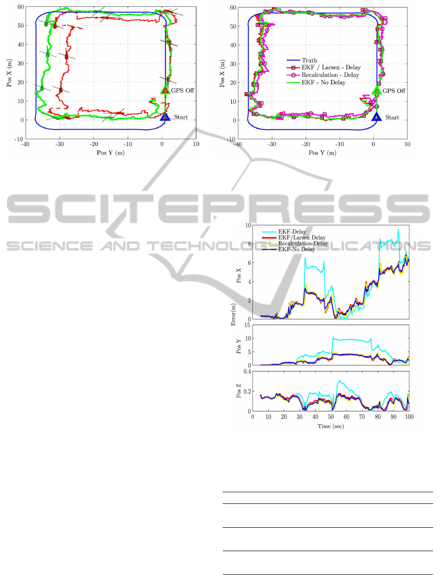
(a) Effects of delay on classic EKF estimate (b) Performance of delayed fusion methods
Figure 5: Comparison of position estimates in the X-Y plane. (a) EKF with (dark-line) and without (light-line) delay on visual
measurements; (b) Recalculation and EKF/Larsen methods in the presence of delayed visual measurements.
5 CONCLUSIONS
In this work, a previously documented VA-INS was
extended by implementing various approaches to han-
dle feature tracking delays in a multi-rate multi-sensor
data fusion process. Simulation experiments were
used together with Monte Carlo analyses to assess the
estimation error and the computational burden of the
methods.
The paper shows that delay caused by image pro-
cessing, if not properly handled in the state estima-
tor, can lead to an appreciable performance degra-
dation. Furthermore, recalculation and sequential
EKF/Larsen restore the estimate accuracy in the pres-
ence of delay, while Alexander method is not a suit-
able solution in this case because of tracking uncer-
tainties. Finally, the results of the paper indicate that
recalculation implies a significant computational bur-
den, while Larsen method is as expensive as the stan-
dard EKF.
This study concluded that Larsen method, for
the present application, provides estimates that have
the same quality and computational cost of the non-
delayed case.
ACKNOWLEDGEMENTS
The authors would like to thank Mehmet Suat Kay
for his help in the development of the feature tracking
code.
Figure 6: Position estimates error in X-Y-Z directions.
Table 3: Monte Carlo simulation results.
Position Velocity Attitude Filter
Method RMSE RMSE RMSE Burden
(m) (m/s) (deg) (sec)
EKF
No Delay
3.7355 0.8173 3.4061 0.0111
EKF
Delay
6.8368 1.1069 3.9330 0.0111
Recalculation
Delay
3.8156 0.8477 3.4397 0.0208
EKF/Larsen
Delay
3.7690 0.8457 3.4336 0.0111
ICINCO2012-9thInternationalConferenceonInformaticsinControl,AutomationandRobotics
400
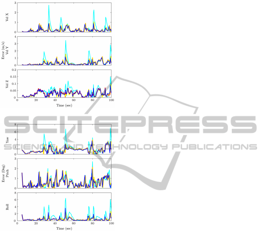
Figure 7: Velocity estimate errors in X-Y-Z directions.
Figure 8: Attitude estimate errors in X-Y-Z directions.
REFERENCES
Alexander, H. L. (1991). State estimation for distributed
systems with sensing delay. SPIE, 1470(1), 103-111.
doi:10.1117/12.44843.
Bonin-Fontand, F., Ortiz, A., and Oliver, G. (2008). Visual
navigation for mobile robots: A survey. Journal of
Intelligent and Robotic Systems, 53(3), 263-296.
Bottasso, C. L. and Leonello, D. (2009). Vision-augmented
inertial navigation by sensor fusion for an autonomous
rotorcraft vehicle. In AHS International Specialists
Meeting on Unmanned Rotorcraft. 324-334.
Calonder, M., Lepetit, V., Strecha, C., and Fua, P. (2010).
Brief: Binary robust independent elementary features.
In 11th European Conference on Computer Vision.
LNCS Springer, 6314(3), 778-792.
Dalgleish, F. R., Tetlow, J. W., and Allwood, R. L. (2005).
Vision-based navigation of unmanned underwater ve-
hicles : a survey. part 2: Vision-basedstation-keeping
and positioning. In IMAREST Proceedings, Part B:
Journal of Marine Design and Operations. 8, 13-19.
Goedeme, T., Nuttin, M., Tuytelaars, T., and Gool, L. V.
(2007). Omnidirectional vision based topological nav-
igation. International Journal of Computer Vision,
74(3), 219-236.
Gopalakrishnan, A., Kaisare, N., and Narasimhan, S.
(2011). Incorporating delayed and infrequent mea-
surements in extended kalman filter based nonlinear
state estimation. Journal of Process Control, 21(1),
119-129.
Jianbo, S. and Tomasi, C. (1994). Good features to track.
In IEEE Computer Society Conference on Computer
Vision and Pattern Recognition. IEEE, 593-600.
Jones, E. S. and Soatto, S. (2011). Visual-inertial nav-
igation, mapping and localization: A scalable real-
time causal approach. The International Journal of
Robotics Research, 30(4), 407-430.
Junker, G. (2006). Pro OGRE 3D Programming. Springer-
Verlag, New York.
Larsen, T. D., Andersen, N. A., Ravn, O., and Poulsen, N.
(1998). Incorporation of time delayed measurements
in a discrete-time kalman filter. In 37th IEEE Confer-
ence on Decision and Control. IEEE, 3972-3977.
Liu, Y. C. and Dai, Q. H. (2010). Vision aided unmanned
aerial vehicle autonomy : An overview. In 3th Inter-
national Congress on Image and Signal Processing.
IEEE, 417-421.
Mourikis, A. I. and Roumeliotis, S. I. (2007). A multi-state
constraint kalman filter for vision-aided inertial navi-
gation. In IEEE International Conference on Robotics
and Automation. IEEE, 3565-3572.
Nister, D., Naroditsky, O., and Bergen, J. (2006). Visual
odometry for ground vehicle applications. Journal of
Field Robotics, 23(1), 3-20.
Pornsarayouth, S. and Wongsaisuwan, M. (2009). Sensor
fusion of delay and non-delay signal using kalman fil-
ter with moving covariance. In ROBIO’09, IEEE In-
ternational Conference on Robotics and Biomimetics.
2045-2049.
Qian, G., Chellappa, R., and Zheng, Q. (2001). Robust
structure from motion estimation using inertial data.
Journal of the Optical Society of America, 18(12),
2982-2997.
Roumeliotis, S. I., Johnson, A. E., and Montgomery, J. F.
(2002). Augmenting inertial navigation with image-
based motion estimation. In ICRA’02, IEEE Interna-
tional Conference on Robotics and Automation. IEEE,
4326-4333.
Tatiraju, S., Soroush, S., and Ogunnaike, B. A. (1999). Mul-
tirate nonlinear state estimation with application to a
polymerization reactor. AIChE Journal, 45(4), 769-
780.
Veth, M. J., Raquet, J. F., and Pachter, M. (2006). Stochastic
constraints for efficient image correspondence search.
Journal of IEEE Transactions on Aerospace Elec-
tronic Systems, 42(3), 973-982.
HandlingDelayedFusioninVision-AugmentedInertialNavigation
401
