
Improved Leader Follower Formation Control of Autonomous
Underwater Vehicles using State Estimation
Umesh Neettiyath and Asokan Thondiyath
Department of Engineering Design, Indian Institute of Technology Madras, Chennai, India
Keywords:
Underwater Robots, Leader Follower Control, Formation Control, AUV, Multirobot Systems.
Abstract:
Multi robot coordination and control for underwater robots is an area of significant importance in many un-
derwater missions. A new approach for leader follower formation control of multi AUV systems is explored
in this paper. The controller estimates the next desired position of the follower robot from the past and current
positions of the leader and follower robots. The control signals are then issued to the follower robot to align it
to the estimated trajectory. This control scheme has the capability to compensate for initial errors and follow
the leader under various operational scenarios. The development of the controller and simulation results for
selected scenarios are presented. The results show that the proposed method is simple and computationally
efficient.
1 INTRODUCTION
Among technologies employed for underwater mis-
sions, Autonomous Underwater Vehicles (AUVs)
play a major role. Their applications range from envi-
ronmental research to military missions. As the com-
plexity of the tasks increases, it becomes necessary
to deploy more than one AUV to accomplish specific
missions. MultiAUV systems are cheaper, more ro-
bust and provides better data quality compared to its
alternatives (Yuh, 2000).
Success in a multi AUV system depends on hav-
ing a good formation control scheme. Researchers
have proposed methods such as behavioral, leader fol-
lower, artificial potential fields, and virtual structures.
Leader follower systems are useful for smaller teams
of robots (Desai et al., 1998; Fahimi, 2009). Much
of the existing controllers try to sense the position of
the follower and tries to align it to the desired path.
This is slow and the convergence to the desired tra-
jectory can be troublesome when there are unexpected
changes in leader trajectory such as dynamic obstacle
avoidance.
The proposed approach on the other hand tries to
estimate its future position and tries to drive the robot
to the desired future state. It is based on l − α con-
troller which is a popular leader follower scheme. It
also has the advantage of being able to operate with
only local information collected from sensors, with
having to rely upon external communication mini-
mally. This is highly desirable in underwater systems
which has to depend on slow noisy acoustic commu-
nication.
2 MODELING OF AUV
In order to represent the motion of an AUV in a 3-
dimensional space, we usually resort to two coordi-
nate frames. The inertial or global coordinate frame
is located at a point of the user’s convenience, for e.g.
mother ship; it is considered to be non-moving. The
body or local coordinate frame is located on the AUV
and it moves along with the AUV.
2.1 Kinematics and Dynamics of AUV
A six dimensional space is required to fully repre-
sent the motion of an AUV in 3-dimensional space.
The position coordinates are represented by η in the
global coordinate frame and velocity coordinates are
represented by ν in the body fixed coordinate frame
(Antonelli et al., 2008; Fossen, 1994). Euler angles
are used to represent orientation. Using above terms,
kinematics of AUV can be written down as
˙
η = J(η)ν (1)
where J(η) is called the Jacobian.
Neettiyath U. and Thondiyath A..
Improved Leader Follower Formation Control of Autonomous Underwater Vehicles using State Estimation.
DOI: 10.5220/0004042104720475
In Proceedings of the 9th International Conference on Informatics in Control, Automation and Robotics (ICINCO-2012), pages 472-475
ISBN: 978-989-8565-22-8
Copyright
c
2012 SCITEPRESS (Science and Technology Publications, Lda.)
The dynamics of AUV can be expressed as (Fos-
sen, 1994; Yuh, 2000)
M
˙
v + C(v)v + D(v)v + g(η)=τ (2)
where M, is the inertia matrix, C (v) is the Cori-
olis and centripetal matrix, D(v) is the damping
matrix and g (η) represents the restoring forces and
moments, which account for the gravitational and
buoyancy forces.τ is the sum of external forces, i.e.
thruster and control plane forces and underwater cur-
rents or other disturbances. The current work does not
take into consideration, the environmental forces.
3 HIERARCHICAL
CONTROLLER FOR AUV
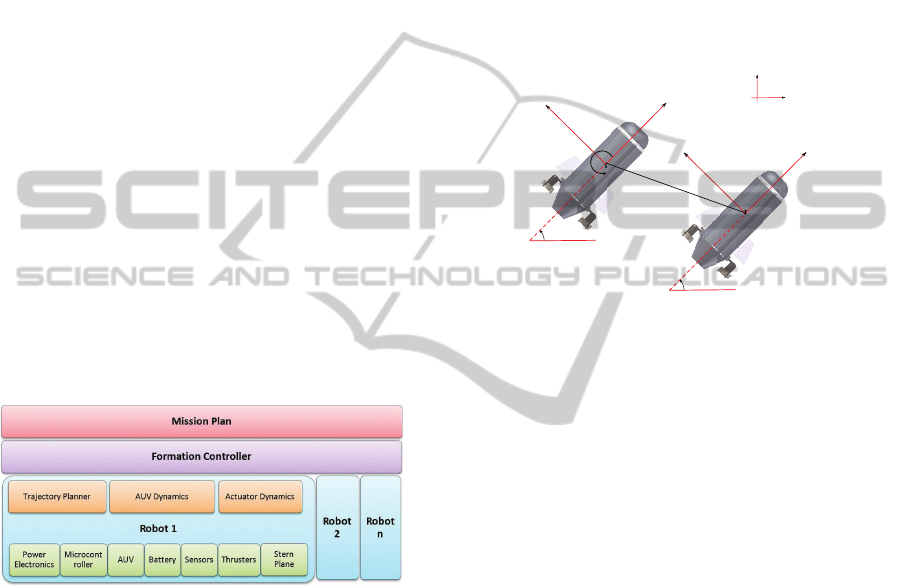
The general control strategy proposed for the AUV
formation is shown in figure 1. The multi layered
hierarchical controller is designed so as to encom-
pass the requirements of various missions and inter-
operability. Another important goal is to minimize
or nullify the amount of data communication between
robots. The method, though proposed for AUVs, may
be used in other types of robots as well; this was not
investigated in the scope of this work.
Figure 1: Multi layered architecture for the controller.
A mission plan specifies all the details required for
the task such as the number of robots, their role in the
formation, desired trajectory for the leader and the in-
flection points, i.e, when there is a predefined change
of formation. These details must be programmed be-
fore the start of mission by a human operator.
Formation controller can reside either globally (as
shown in figure 1) or in the leader AUV. It gets acti-
vated only at an inflection point to change the forma-
tion type or parameters. Otherwise, the robots follow
their leader without any explicit communication.
The two lowest layers functions in all the AUVs.
The upper layer takes the commands from the forma-
tion controller and initiates actuation. The trajectory
planner takes into consideration all the dynamic and
kinematic parameters to calculate the control signals
for the low level subsystems. The lower layer inside
the vehicle contains all physical resources of the ve-
hicle including sensors, actuators and the electronic
circuitry.
3.1 Improved l − α Controller
The proposed improved l − α controller, forms part
of the trajectory planner in the follower robot. It takes
the pose information from the leader and follower and
process them to estimate the future positions. For this
purpose, a time history of a number of previous posi-
tions are stored in the controller.
y
1
x
1
ψ
1
O
1
α
d
o
y
x
global
y
2
x
2
ψ
2
O
2
l
d
Follower AUV
Leader AUV
Figure 2: Parameters for a leader follower scheme.
This can be explained using figure 2. The leader
AUV is located at O
1
and moves along a predefined
trajectory. The follower AUV is located at O
2
and
tries to follow the leader. The line O
1
O
2
is expected to
be maintained at length l
d
and at an angle α
d
with the
local x axis of the leader. To achieve this, the desired
next position of the follower is determined from the
expected next position of the leader as
η
2d
(t + 1)=η
1
(t + 1)+Tr(ψ(t + 1))Tr(α
d
)
l
d
0
(3)
where Tr(ψ(t +1)) denotes the rotational transforma-
tion matrix., defined as(Xiang et al., 2009)
Tr(χ)=
⎡
⎣
cosχ − sinχ 0
sinχ cosχ 0
001
⎤
⎦
(4)
3.2 Next State Estimation
The controller estimates the next positions of the
leader and follower as shown in figure 3. The robot
is assumed to have a constant velocity in all direc-
tions for interval of time from the past measured time
instant to the next time instant to be measured. The
sampling time is also assumed to be constant. The
expected next position of the leader robot is estimated
using equation 5.
,PSURYHG/HDGHU)ROORZHU)RUPDWLRQ&RQWURORI$XWRQRPRXV8QGHUZDWHU9HKLFOHVXVLQJ6WDWH(VWLPDWLRQ

x
1
(t − 1) y
1
(t − 1)
x
1
(t) y
1
(t)
x
1
(t + 1) y
1
(t + 1)
x
2
(t − 1) y
2
(t − 1)
x
2
(t) y
2
(t)
x
2a
(t + 1) y
2a
(t + 1)
x
2d
(t + 1) y
2d
(t + 1)
l
d
α
d
Follower AUV
Leader AUV
Figure 3: Estimation of next position of leader and follower.
η
1
(t + 1)=(η
1
(t) − η
1
(t − 1)) + η
1
(t) (5)
Similarly, we can estimate the next position
(henceforth referred to as the driven position) of the
follower AUV as
η
2a
(t + 1)=(η
2
(t) − η
2
(t − 1)) + η
2
(t) (6)
3.3 Follower Control
The methodology used to control the follower AUV
can be explained using figure 4. The follower robot
is now left with two future positions - the driven po-
sition (D(x
2a
(t + 1), y
2a
(t + 1))), which it will reach
if no correction is done and the desired position
(G(x
2d
(t +1),y
2d
(t +1))), which is the ideal position.
Now the task of the controller is to issue a correction
signal so that the AUV is driven from the current po-
sition (C(x
2
(t),y
2
(t))) to the desired position within
the specified time.
C
ψ
Driven
(t)
ψ
Desired
(t)
D
(x
2a
(t + 1), y
2a
(t + 1)
G
(x
2d
(t + 1), y
2d
(t + 1)
(x
2
(t),y
2
(t)
Figure 4: Follower is driven towards the desired position.
The distance to be travelled in each case is calcu-
lated as the Cartesian distance from current position
to next positions as given in equations 7 and 8.
d
Driven
=
((x
2a
(t + 1) − (x
2
(t))
2
+((y
2a
(t + 1) − y
2
(t))
2
(7)
d
Desired
=
((x
2d
(t + 1) − (x
2
(t))
2
+((y
2d
(t + 1) − y
2
(t))
2
(8)
Based on this, a correction term for linear velocity of
the follower is calculated as
δv = K
v
(d
Driven
− d
Desired
)/Δt (9)
where Δt is the time step between two states.
Similarly, the desired and driven yaw(heading) is
calculated from the position values as
tanψ
Driven
=
y
2a
(t + 1) − y
2
(t)
x
2a
(t + 1) − x
2
(t)
(10)
tanψ
Desired
=
y
2d
(t + 1) − y
2
(t)
x
2d
(t + 1) − x
2
(t)
(11)
The correction term for angular velocity is calcu-
lated as
δω = K
w
(ψ
Driven
− ψ
Desired
)/Δt (12)
We get the new desired values of velocity by
adding the correction values to the previous values
(equation 13).
v(t)=v(t − 1)+δv (13)
ω(t)=ω(t − 1)+δω (14)
These correction values are updated to the low
level controller of the robot.
4 IMPLEMENTATION
For simulation purposes, a vehicle system containing
two AUVs is considered. The leader AUV is consid-
ered to be an ideal vehicle that follows the assigned
trajectory without position or velocity error. The tra-
jectory is generated using the method given in section
4.1. The follower AUV is driven by the previously
described controller. It tries to follow the leader by
maintaining the l and α values.
4.1 Trajectory Generation
Cartesian space trajectory planning is employed for
the position variables in the global coordinate frame.
For planar trajectory planning, out of the 3 degrees of
freedom (x, y and yaw) 2 are selected (x and y) and a
sixth order time parametrised function is defined for
each of them. This ensures that the path is continuous
and differentiable. If the position variable is ζ, the
polynomial defined is
ζ(t)=a
i1
+ a
i2
t + a
i3
t
2
+ a
i4
t
3
+ a
i5
t
4
+ a
i6
t
5
(15)
Differentiating the polynomial, we get the velocity
relation as:
˙
ζ(t)=a
i2
+ 2a
i3
t + 3a
i4
t
2
+ 4a
i5
t
3
+ 5a
i6
t
4
(16)
Three points are selected along the trajectory and
the desired position and velocity at these points are
,&,1&2WK,QWHUQDWLRQDO&RQIHUHQFHRQ,QIRUPDWLFVLQ&RQWURO$XWRPDWLRQDQG5RERWLFV
calculated. These values can be substituted into equa-
tions 15 and 16 and they are solved to get the param-
eters of the trajectory.
5 RESULTS
The controller described above was tested through
simulations for dynamic conditions. Simulations
were conducted for various initial errors (initial po-
sition or yaw) and for various values of l and α and
performance was studied.
Initially, the leader AUV was commanded a
straight line trajectory. The desired l was set as 2 and
desired α was set as π/2. The gain values were set as
1 and 10 for Kv and Kw respectively. The system was
simulated for different initial position errors i.e, 1m,
2m at different angles.
0 10 20 30 40 50 60 70 80 90 100
0
0.5
1
1.5
2
2.5
3
3.5
4
x,Surge
y,Sway
Plot of the AUV path
Follower Path : Initial error 1m
Follower Path : Initial error 2m
Follower Path : Initial error 1m
Follower Path : Zero initial error
Leader Path
Figure 5: Simulation results for formation with initial posi-
tion error.
As observed in figure 5 that relatively small errors
in the initial position of the follower AUV is corrected
and the follower trajectory exponentially converges to
the desired trajectory. It can be seen that as error in-
creases, settling time increases.
Another set of simulations were done with a more
complex trajectory to check the performance under
conditions with an initial yaw error. The formation
parameters and control gains were kept as the same
as the previous case. The results are shown in figure
6. It was seen that the AUV could converge to desired
trajectory despite considerable initial yaw errors.
0 5 10 15 20 25 30 35 40
0
5
10
15
20
25
30
35
40
x,Surge
y,Sway
Plot of the AUV path
Leader Path
Follower : Initial yaw = π/12
Follower : Initial yaw = π/4
Follower : Initial yaw = π/2
Figure 6: Simulation results for formation with initial yaw
error.
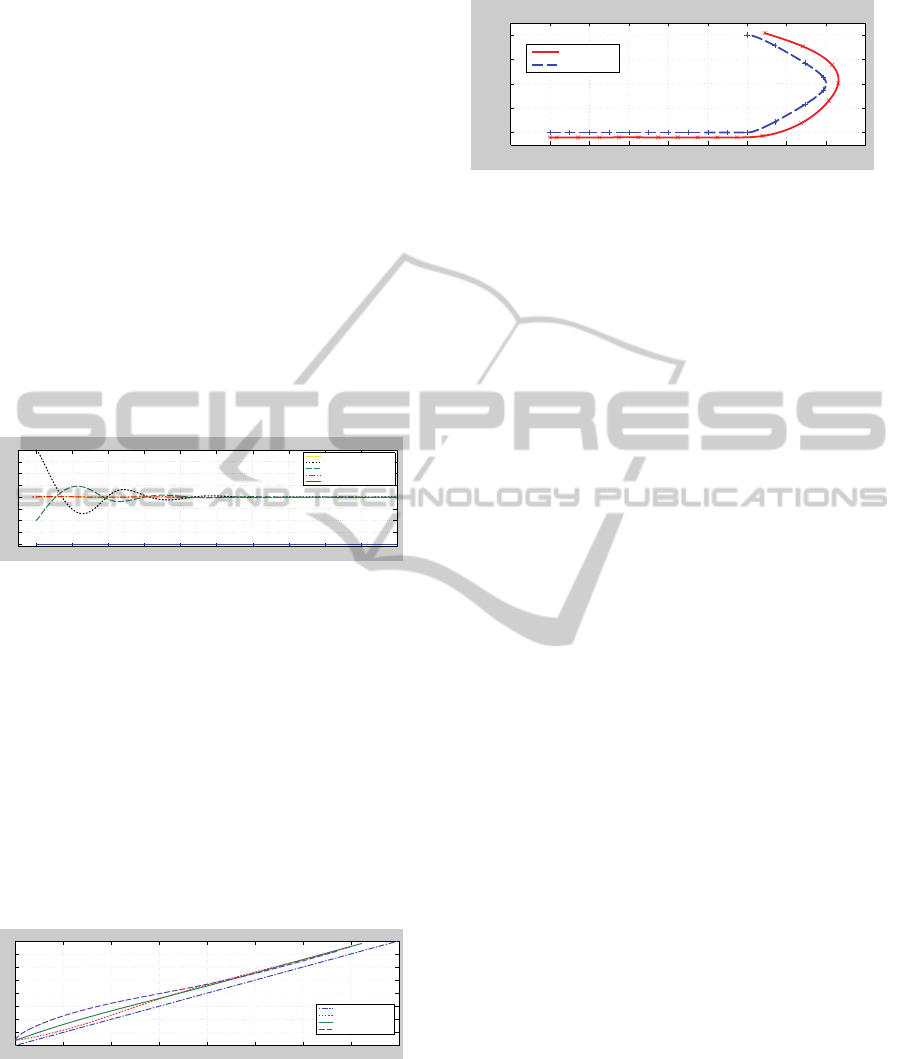
In order to check the effectiveness of the con-
troller, a blended path is given to the leader. The path
consisted of a curve fitted to the end of a straight line
trajectory at end of which the robot will make a 180
degree turn. These paths are generated using tech-
−10 0 10 20 30 40 50 60 70 80
−100
−90
−80
−70
−60
x,Surge
y,Sway
Plot of the AUV path for a complex trajectory
Follower Path
Leader Path
Figure 7: Simulation results for AUV following blended
paths.
niques mentioned in section 4.1. This made it sure
that there is no sudden jump in velocity of the robot.
The simulation results shown in figure 7 showed
that the AUV is able to follow the complex trajectory
easily, except at changeover points where the AUV
took some time to align to the trajectory.
During simulations, it was observed that the gains
Kv and Kw have a large impact in stabilising the tra-
jectory. Therefore careful gain tuning is required.
This can be treated as a multivariate optimisation
problem, which is a possible extension of this work.
6 CONCLUSIONS
An improved formation control strategy is presented
for the control of a multi AUV system which tries to
estimate the future states of the robots. The proposed
algorithm is found to satisfy the requirements of for-
mation control under various situations. Further ef-
forts to implement this controller in real time is under
way.
REFERENCES
Antonelli, G., Fossen, T. I., and Yoerger, D. R. (2008). Un-
derwater robotics. In Siciliano, B. and Khatib, O.,
editors, Springer Handbook of Robotics, chapter 44,
pages 987–1008. Springer Berlin Heidelberg, Berlin,
Heidelberg.
Desai, J. P., Ostrowski, J., and Kumar, V. (1998). Control-
ling formations of multiple mobile robots. In Robotics
and Automation, 1998. Proceedings. 1998 IEEE Inter-
national Conference on, volume 4, pages 2864–2869
vol.4. IEEE.
Fahimi, F. (2009). Autonomous Robots Modeling, Path
Planning, and Control. Springer.
Fossen, T. I. (1994). Guidance and control of ocean vehi-
cles. Wiley.
Xiang, X., Lapierre, L., Jouvencel, B., and Parodi, O.
(2009). Coordinated path following control of mul-
tiple nonholonomic vehicles. In OCEANS 2009 - EU-
ROPE, pages 1 –7.
Yuh, J. (2000). Design and control of autonomous underwa-
ter robots: A survey. Autonomous Robots, 8(1):7–24.
,PSURYHG/HDGHU)ROORZHU)RUPDWLRQ&RQWURORI$XWRQRPRXV8QGHUZDWHU9HKLFOHVXVLQJ6WDWH(VWLPDWLRQ
