Applying Hyperbolic Wavelets in Frequency Domain Identification
Alexandros Soumelidis
1
, J´ozsef Bokor
1
and Ferenc Schipp
2
1
Systems and Control Laboratory, Computer and Automation Research Institute, Budapest, Hungary
2
Department of Numerical Analysis, E¨otv¨os Lor´and University, Budapest, Hungary
Keywords:
System Identification, Discrete–time Systems, Frequency–domain Representations, Wavelets, Hyperbolic
Geometry.
Abstract:
The paper elaborates a hyperbolic wavelet construction for representing signals in the Hardy space H
2
on the
unit disc. An efficient computing scheme based on the matrix form of the representation is worked out. The
wavelet coefficients can be computed on the basis of discrete time–domain measurements. This wavelet is
used to reconstruct poles of functions in H
2
as the basis of nonparametric frequency–domain identification of
discrete–time signals and systems.
1 INTRODUCTION
Representations of discrete-time signals and systems
in the frequency domain are used in many fields of
science and technology, e.g. in detection and changes
in systems, system identification, and control design.
The stable representations of signals and systems of
finite energy result in complex analytic functions de-
fined on the unit disc of the Hardy space H
2
. The
identification of H
2
signals is usually based on phys-
ical measurements in the time–domain. Convenient
methods for system identification can be obtained in
the case when an orthogonal basis of the space H
2
is
used. A well-known orthonormal basis in H
2
is the
trigonometric system that forms the basis of classi-
cal Fourier–transform representations and associated
identification methods. Orthogonal bases can also be
generated by rational functions and this concept leads
to rational orthogonal bases (ROBs) that have gained
great significance besides H
2
also in H
∞
system iden-
tification (Heuberger et al., 2005). Application of
ROBs requires a priori information on the locations
of system poles. This paper elaborates a method to
obtain representations of H
2
functions that does not
use strict a priori assumptions. A promising opportu-
nity to realize this arises from some wavelet-type con-
struction that utilize the hyperbolic geometry gener-
ated by the so-called Blaschke functions. The goal is
to apply hyperbolic wavelet methods to identify poles
of functions in H
2
.
2 RATIONAL ORTHOGONAL
BASES
The Blaschke function in H
2
(D) is defined as
B
b
(z) :=
z−b
1−bz
(z ∈ C,b ∈D),
where b is called the parameter of the Blaschke-
function. The parameter b is identical to the zero and
b
∗
= 1/b is the pole of B
b
.
The most important feature of the Blaschke func-
tion is that B
b
: T → T and B
b
D → D are bijections,
as a consequence the Blaschke functions to be inner
functions in the space H
2
(D).
The discrete Laguerre-system is complete or-
thonormed system in H
2
(D) defined by
φ
n
(z) =
p
1−|b|
2
1−bz
B
n
b
(z), (n = 0,1, . . .).
If the pole locations of the system are exactly
known one obtains finite rational representations
(Soumelidis et al., 2002b). Rational orthogonal bases
have intensively been discussed in the context of H
2
and H
∞
identification of systems (Heuberger et al.,
2005), and efficient methods have been elaborated
that solved the identification problem in the case when
— at least approximately — the pole locations are
known. Special attention paid on the problems of pole
selection and validation (Bokor et al., 1999; e Silva,
2005) as well as methods have been found to refine
the pole locations starting from an approximate place-
ment (Soumelidis et al., 2002a), however the general
problem identifying poles has not been solved so far.
532
Soumelidis A., Bokor J. and Schipp F..
Applying Hyperbolic Wavelets in Frequency Domain Identification.
DOI: 10.5220/0004043705320535
In Proceedings of the 9th International Conference on Informatics in Control, Automation and Robotics (ICINCO-2012), pages 532-535
ISBN: 978-989-8565-21-1
Copyright
c
 2012 SCITEPRESS (Science and Technology Publications, Lda.)

3 HYPERBOLIC WAVELETS
It is known that the Blaschke functions form a group
with respect to the function composition, i.e. (B
b
1
◦
B
b
2
)(z) := B
b
1
(B
b
2
(z)) . In the set of the parame-
ters B := D ×T let us define the operation induced
by the function composition in the following way
B
b
1
◦B
b
2
= B
b
1
◦b
2
. The (B, ◦) results in a group iso-
morphic with the group group of the Blaschke func-
tions. The neutral element of the group (B, ◦) is e :=
(0,1) ∈ B and the inverse element of b = (b,ε) ∈ B is
b
−1
= (−bε,ε).
This group can be associated with the congruence
transforms of the Poincar´e model of the hyperbolic
geometry (see e.g. (Ahlfors, 1973)). It can be proved
that the map
ρ(z
1
,z
2
) :=
|z
1
−z
2
|
|1−z
1
z
2
|
= |B
z
1
(z
2
)|
(B
z
1
:= B
(z
1
,1)
,z
1
,z
2
∈D)
is a metric on D, called pseudohyperbolic metric
(Ahlfors, 1973). Moreover the Blaschke functions B
b
(b ∈D) are isometries with respect to this metric, i.e.
ρ(B
b
(z
1
),B
b
(z
2
)) = ρ(z
1
,z
2
)
(b ∈ D,z
1
,z
2
∈ D).
It is also well–known that the Hardy space H :=
H
2
(D) is Hilbert space with respect to the inner prod-
uct
hf,gi :=
1
2π
Z
π
−π
f(e
it
)g(e
it
)dt ( f,g ∈ H),
and the power functions h
n
(z) := z
n
(z ∈ C,n ∈ N)
form an orthonormal basis in the space. By defining
the multiplier function
R
b
(z) :=
p
ε(1−|b|
2
)
1−bz
(z ∈ D,b := (b, ε) ∈ B := D ×T),
introduce the mapping
U
b
f := R
b
−1
f ◦B
b
−1
(b ∈ B, f ∈ H). (1)
(U
b
,b ∈ B) can be considered as a unitary represen-
tation of the group (B,◦) on the Hilbert space H with
properties
(i) U
b
1
(U
b
2
f)) = U
b
1
◦b
2
f (b
1
,b
2
∈ B, f ∈ H),
(ii) kU
b
fk = kfk ( f ∈ H,b ∈B),
(iii) b →U
b
f ∈ H ( f ∈ H,b ∈ B) is continuous.
See for proofs in (Pap and Schipp, 2006), and an
introduction to the unitary group representations in
(Wawrzy´nczyk, 1984). From the properties (i) to (iii)
follows that U
b
maps any complete orthogonal sys-
tem in H into complete orthogonal system in the same
space. Particularly the system
L
b
n
:= U
b
−1
h
n
(n ∈ N,b := (b, 1) ∈ B)
form an orthogonal basis in H that is called discrete
Laguerre system.
The unitary group representations allow us to in-
troduce the concept of the wavelets in the Hilbert
space H (Goupillaud et al., 1984), (Meyer, 1990), and
(Daubechies, 1992). The continuous wavelet trans-
form on a function f ∈ L
2
(R) is formed by taking
translation and dilation of a function ψ named the
mother wavelet; the integral operator with the kernel
ψ
pq
(x) :=
ψ((x−q)/p)
√
p
, x ∈R,
p ∈ (0,∞),q ∈R is called wavelet transform:
(W
ψ
f)(p,q) :=
1
√
p
Z
R
f(x)ψ

x−q
p

dx =
=hf,ψ
pq
i ( f ∈ L
2
(R)),
where h·, ·i means the inner product of the Hilbert-
space L
2
(R). Using the unitary representation U
b
(b ∈ B) defined by (1) one obtains
(W
ϕ
f)(b) = hf,U
b
ϕi ( f, ϕ ∈ H
2
(D),b ∈ B),
where h·, ·i is the scalar product in the Hardy space
H
2
(D). This construction can be referred as Blaschke
or hyperbolic wavelet.
Particularly the hyperbolic wavelets generated by
the power–functions
ε
n
(t) := e
int
(n ∈ Z,t ∈ R),
can be interpreted as the Laguerre–Fourier coeffi-
cients, i.e. the Laguerre representation of any func-
tion f ∈ H can be considered as a hyperbolic wavelet
transform.
Any function f ∈ H can be expressed in the
trigonometrical system in the form
f =
∞
∑
n=0
b
f(n)ε
n
(t),
where
b
f(n) := hf,ε
n
i (n ∈ N)
is the n-th trigonometric Fourier–coefficients of the
function f . Consequently the Fourier–coefficients of
F
b
:= U
b
f =
∞
∑
n=0
b
f(n)U
b
ε
n
can be obtained as
b
F
b
(m) :=hU
b
f, ε
m
i =
=
∞
∑
n=0
hU
b
ε
n
,ε
m
i
b
f(n) =
∞
∑
n=0
u
mn
(b)
b
f(n),
ApplyingHyperbolicWaveletsinFrequencyDomainIdentification
533

where u
mn
(b) = hU
b
ε
n
,ε
m
i ((m,n) ∈ N
2
) form the
matrix of the representation U
b
in the trigonometri-
cal basis. By introducing the matrix
U
b
= [u
mn
(b)]
(m,n)∈N
2
,
the mapping f → F
b
can be expressed in the space of
the Fourier–coefficients with the matrix–transform
b
F
b
= U
b
b
f ( f ∈ H,U
b
= {u
mn
(b)}). (2)
Since the transform is unitary, i.e. U
b
−1
= U
−1
b
= U
∗
b
,
the elements
u
mn
(b) = hU
b
ε
n
,ε
m
i = u
mn
(b) (m,n ∈ N).
can be expressed by the Jacobi–polynomials, i.e.
u
mn
(b) =
= (−1)
m
p
1−r
2
e
i(n−m)α
r
|n−m|
P
(0,|n−m|)
min{m,n}
(2r
2
−1).
The Fourier–coefficients in
b
f correspond to
discrete–time signal data points that can be in-
terpreted as the uniformly sampled form of the
continuous–time physical signals. Computation of
the elements in U
b
can be performed by using recur-
sions for any parameter selection b ∈ B, and in ad-
vance to taking the measurements.
4 IDENTIFYING POLES
Suppose that the system under consideration contains
only a single pole of multiplicity 1, in this case the
conjugated Laguerre–Fourier coefficients are given as
b
F
b
(m) = L
b
m
(a), and the quotients
q
m
(b) =
b
F
b
(m+ 1)
b
F
b
(m)
= B
b
(a) (m ∈ N),
form a constant sequence and its elements equal to a
Blaschke function applied to a. This fact can be used
to identify the position of inverse pole a,
a = B
b
−1
(q
m
(b)),
where B
b
−1
is the inverse of B
b
, i.e. a is given by
applying a hyperbolic transform corresponding to the
inverse group element belonging to b.
This concept can be extended to multiple poles, it
will be shown that in the case of multiple poles there
exist a region D
i
∈ D where the sequence of the quo-
tients generated by the conjugated Laguerre–Fourier
coefficients converge. A theorem can be set up as fol-
lows:
Theorem 1. For any rational function f in any point
b of D the limit
(Q f)(b) := lim
n→∞
q
m
(b) ( f ∈ R)
exists, and
(Q f)(b) = B
b
(a
i
), b ∈ D
i
(i = 1,2, . ..,P).
In the case of poles of multiplicity 1 for the speed of
convergence the estimation
|q
m
(b) −B
b
(a
i
)| = O(q
n
i
) (n ∈ N,b ∈D
i
,q
i
< 1)
can be given.
The proof can be found in (Schipp and Soumelidis,
2011).
The result of Theorem 1 can be used to reconstruct
the poles of function f by
B
−1
b
((Q f)(b)) = a
i
(b ∈D
i
,i = 1, 2,··· ,P). (3)
By this way all the poles can be reconstructed that
possess nonempty region, i.e D
i
6=
/
0. The procedure
goes like this:
1. Estimation of the Laguerre–Fourier coefficients
belonging to parameter b based on measurements.
2. Reconstruction the poles as a limit of quotients of
consecutive Laguerre–Fourier coefficients.
The estimation of the Laguerre–Fourier coefficients
of function f with parameter b can efficiently be com-
puted according to the form (2) applied on the time–
domain signal measurements. Finding multiple poles
can be done by selecting a sequence of parameters b
arranged randomly or in arbitrary order.
5 A NUMERICAL EXAMPLE
The identification of the poles of a simulated function
is presented. The set of (inverse) poles belonging to
the function is {a
1
= 0.8,a
2,3
= 0.8 ∗e
±i
π
4
} with the
associated residues {λ
1
= 1.5,λ
2,3
= 1}.
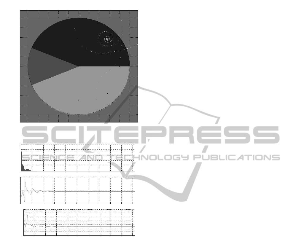
Figure 1 presents a visualization of the iteration
processes for finding specific poles. The sequence
given by (3) is drawn in the complex plane by white
points. The sequence converges towards pole des-
ignated by a
2
. The convergence can be checked on
the lower two diagrams in Figure 2where the absolute
value and the phase of the sequences against the in-
dices can be seen. The upper diagram in these figures
depicts the absolute value of the Laguerre-Fourier co-
efficients belonging to the specific selection of b. The
reconstruction error – defined as a root-mean-square
difference – is in the magnitude 10
−5
...10
−7
.
Figure 1 also presents the regions D
i
that belongs
to the poles a
i
. Poles a
1
and a
3
can be identified by
selecting parameter b within the other two regions.
ICINCO2012-9thInternationalConferenceonInformaticsinControl,AutomationandRobotics
534

−1 −0.8 −0.6 −0.4 −0.2 0 0.2 0.4 0.6 0.8 1
−1
−0.8
−0.6
−0.4
−0.2
0
0.2
0.4
0.6
0.8
1
error=6.83196e−007
b →
a
1
a
2
a
3
Figure 1: Finding pole a
2
.
0 50 100 150 200 250 300 350 400 450 500
0
0.2
0.4
0.6
0.8
1
abs[q(1)]=0.927487 abs[q(2)]=0.955407 abs[q(3)]=0.805005
0 50 100 150 200 250 300 350 400 450 500
0.5
1
1.5
abs(Q) = 0.955407 / err = 1.37539e−007
0 50 100 150 200 250 300 350 400 450 500
−0.7
−0.6
−0.5
−0.4
−0.3
−0.2
−0.1
0
arg(Q)=−0.454192
[x π]
Figure 2: Modulus of the L-F coefficients, modulus and
phase of sequence q
n
.
6 CONCLUSIONS
A hyperbolic wavelet concept for representing signals
belonging to the space of functions H
2
on the unit
disc has been constructed, and an efficient comput-
ing scheme based upon the matrix form of the rep-
resentation has been elaborated. The wavelet coeffi-
cients can be computed on the basis of discrete time–
domain measurements. The wavelet construct can be
used in reconstructing poles belonging to functions
in H
2
(D), which forms the basis of nonparametric
frequency–domain identification of discrete–time sig-
nals and systems.
ACKNOWLEDGEMENTS
This work is supported by the Control Engineering
Research Group of HAS at Budapest University of
Technology and Economics. The European Union
and the European Social Fund have provided finan-
cial support to the project under the grant agreement
no. T
´
AMOP-4.2.1./B-09/1/KMR-2010-0003.
REFERENCES
Ahlfors, L. (1973). Conformal invariants. McGraw-Hill,
New York.
Bokor, J., Ninness, B., e Silva, T. O., Van den Hof, P.
M. J., and Wahlberg, B. (1999). Selection of poles in
GOBF models. In Modelling and Identification with
Orthogonal Basis Functions, Workshop notes of a pre-
conference tutorial presented at the 14th IFAC World
Congress, Beijing, China. Chapter 5.
Daubechies, I. (1992). Ten lectures on wavelets.
CBMS/NSF Series in Applied Mathematics; 61.
SIAM, Philadelphia, Pennsylvania.
e Silva, T. O. (2005). Pole selection in GOBF mod-
els. In Heuberger, P. S. C., Van den Hof, P. M. J.,
and Wahlberg, B., editors, Modelling and Identifica-
tion with Rational Orthogonal Basis Functions, chap-
ter 11, pages 297–336. Springer Verlag.
Goupillaud, P., Grossmann, A., and Morlet, J. (1984).
Cycle-octave and related transforms in seismic signal
analysis. Geoexploration, 25:85–102.
Heuberger, P. S. C., Van den Hof, P. M. J., and Wahlberg,
B. (2005). Modelling and Identification with Rational
Orthogonal Basis Functions. Springer Verlag, New
York.
Meyer, Y. (1990). Ondolettes et Operateurs. Hermann, New
York.
Pap, M. and Schipp, F. (2006). The voice transform on
the Blaschke group I. Pure Mathematics and Appli-
cations, 17(3-4):387–395.
Schipp, F. and Soumelidis, A. (2011). On the Fourier coef-
ficients with respect to the discrete Laguerre system.
Annales Univ. Sci. Budapest, Sect. Comput., 34:223–
233.
Soumelidis, A., Pap, M., Schipp, F., and Bokor, J. (2002a).
Frequency domain identification of partial fraction
models. In Proceedings of the15th IFAC World
Congress, page on CD, Barcelona, Spain.
Soumelidis, A., Schipp, F., and Bokor, J. (2002b). Fre-
quency domain representation of signals in rational
orthogonal bases. In Proc. of the 10th Mediterranean
Conference on Control and Automation, page on CD,
Lisboa, Portugal. MED’2002.
Wawrzy´nczyk, A. (1984). Group Representations and Spe-
cial Functions. Mathematics and Its Applications.
D. Reidel Publishing Comapany, Dordrecht, Boston,
Landcaster.
ApplyingHyperbolicWaveletsinFrequencyDomainIdentification
535