Self–Scheduled
∞
H
Control of a Wind Turbine
A Real Time Implementation
Florin Sebastian Tudor, Dumitru Popescu and Dan Stefanoiu
”Politehnica” University of Bucharest, Department of Automatic Control and Computer Science
313 Splaiul Independentei, 060042, Bucharest, Romania
Keywords: Wind Power, Renewable Energy, Robust, Control, Gain-scheduling, LPV, Modeling, Real Time
Implementation.
Abstract: This paper is concerned with the design of robust gain-scheduled controllers with guaranteed H
∞
performance for a horizontal axis wind turbine (HAWT) with variable-speed and fixed-pitch. The control
problem in terms of Linear Parameter-Varying (LPV) plants is stated and the theoretical background of the
design method is given. Due to some interesting properties outlined in this paper, the synthesis problem is
reduced to solving off-line a finite-dimensional set of Linear Matrix Inequalities (LMIs), making the
controller suited for real-time applications. The computed LPV controller focuses on multiple objectives
such as mechanical fatigue reduction, speed regulation and mode stabilization with simultaneously
maximizing energy capture. The performances obtained through this control method are discussed and
presented by means of a set of simulations. A real-time control algorithm for the large-scale wind turbines is
also proposed.
1 INTRODUCTION
Nowadays, the development of electrical power
generation from wind currents is a big concern for
the society energy issue as well as for the
management of electrical power systems. As wind
turbines prove to be one of the cheapest, cleanest
and most efficient sources of energy, it has become
of great necessity to focus on complex algorithms to
meet with multiple objectives.
The wind is the main energy source and, thus, it is
of great importance to determine the characteristics
of the wind currents passing through the turbine
rotor. The stochastic nature of the wind determines
the necessity of a wind turbine to be able to work
under different wind velocities.
In order to keep the performance within these
conditions, controllers have to be designed and
implemented. Various control synthesis options have
been applied in response to wind turbine control
problem such as PID controllers, LQG controllers or
fuzzy logic. The classical control structures proved
to be simple and robust but most of the times they
require the implementation of multiple control loops,
in order to accomplish multiple control objectives.
An interesting approach is the formulation of gain
scheduling control. These techniques are largely
used since they tackle the control of nonlinear
systems with the tools of the well-known linear
control theory. In the context of Linear Parameter-
Varying (LPV) systems, the design follows a
procedure similar to H
∞
synthesis.
Due to the development of the power converters
and microcontrollers, a wind turbine can operate in a
variable-speed mode, making it suitable for
optimization. Thus, in this research a variable-speed
fixed pitch wind turbine has been analyzed. The
main goal was to design an LPV controller with
guaranteed H
∞
- like performance, ensuring closed-
loop stability.
This paper is structured as follows. Section 2
presents some theoretical aspects of the gain-
scheduling problem and the synthesis procedure. In
Section 3, an LPV model is determined in order to
design the self-scheduled H
∞
controller. A set of
simulations confirms the robustness of the system.
Finally, the possibility of a digital implementation is
discussed.
402
Sebastian Tudor F., Popescu D. and Stefanoiu D..
Self-scheduled H#INF# Control of a Wind Turbine - A Real Time Implementation.
DOI: 10.5220/0004045904020411
In Proceedings of the 9th International Conference on Informatics in Control, Automation and Robotics (ICINCO-2012), pages 402-411
ISBN: 978-989-8565-21-1
Copyright
c
 2012 SCITEPRESS (Science and Technology Publications, Lda.)

2 THEORETICAL FRAMEWORK
2.1 LPV Models for Nonlinear Systems
It is a known fact that in control engineering, most
of the dynamical systems are nonlinear.
Nevertheless, they can be approximated as LTI
systems around the equilibrium or some operating
points. Then, by seeing the nonlinear dynamical
system as a collection of LTI behaviors
corresponding to different operating points, and
using some well chosen variables to perform
switching between them, one can have an
approximation of the global behavior. Such a
modeling approach, detailed in (Tóth, 2010), defines
an LPV system. In the context of gain scheduling
techniques, LPV models form a well known class of
models, with practical applications in many fields of
control engineering, e.g. modeling, system
identification, and control.
An LPV system can be described by a state-space
realization:
(
)
(
)
( ) ( )
:
( ) ( ) ( ) ( ) ( )
( ) ( ) ( ) ( ) ( )
zw
t t t t t
t t t t t
= ⋅ + ⋅
= ⋅ + ⋅





x
θ x θ w
T
z θ x θ w
&
A B
C D
, (1)
where
R
nx
∈
x
is the state vector,
R
nz
∈
z
is the
output or the error signal,
R
nw
∈w is the input
(disturbance),
θ
R
n
∈θ
is the time-varying parameter
vector, and
(
)
(
)
(
)
(
)
, , ,
⋅ ⋅ ⋅ ⋅
A B C D
are continuous
functions, evaluated at the operating points
θ
. When
freezing
(
)
t
θ
to some given value
0
θ
, the LPV
system (1) becomes an LTI system of transfer
function:
( ) ( ) ( )
( )
( ) ( )
1
0 0 0 0zw
s s
−
= − +T
θ I θ θ θ
C A B D
.
Note that
(
)
t
θ
as well as its rate of variation
(
)
t
θ
&
are assumed bounded, that is
(
)
( ), ( ) , 0
t t t
∈ Θ × Θ ∀ ≥
θ θ
&
%
, (2)
(
)
(
)
{
}
( ) ( )
{ }
: , 1, , , 0
: , 1, , , 0
vi
vi
t t i r t
t t i r t
Θ = ≤ = ∀ ≥
Θ = ≤ = ∀ ≥
θ : θ θ
θ : θ θ
K
& & %
%
K
,
which means that
( )
t
θ
is valued in the polytope
Θ
,
a bounded and connected set, with vertices in
, 1, ,
vi
i r
=θ K
; similarly,
( )
t
θ
&
is valued in
Θ
%
,
having the same properties as
Θ
.
2.2 Stability and Performance
Stability of the LPV system defined in (1) can be
established by finding a parameter-dependent
Lyapunov function. This approach leads to the
concept of parameter-dependent quadratic (PDQ)
stability introduced in (Wu et al., 1996). It was also
shown that the PDQ stability condition implies the
autonomous LPV system
(
)
( ) ( ) ( )
t t t
= ⋅x
θ x
&
A
is
uniformly exponentially stable.
The performance of a closed-loop system can be
characterized in several ways. In LTI theory, the
performance is commonly measured by the induced
2
norm
−L
, using the well known Bounded Real
Lemma (BRL). This famous lemma can be extended
for an LPV system as a Linear Matrix Inequality
(LMI) problem, as stated in (Becker and Packard,
1994), (Wu et al., 1996), (Apkarian and Adams,
1998), with quadratic parameter-dependent
Lyapunov functions:
(
)
(
)
,
T
=x
θ x P θ x
V
, (3)
where
(
)
: R
nx nx
×
Θ →P θ
. In order for the problem
to have a solution to the extended problem, the time-
varying parameter
( )
t
θ
has to be bounded, as in (2).
The induced
2
norm
−L
for the LPV system (1) is
defined as:
( )
2
2
2
2
,
: sup sup
zw
∈Θ×Θ
=
∈
θ θ
z
T
w
w
&
%
L
, (4)
where
2
L
denotes the space of the Lebesgue square
integrable vector functions with the corresponding
norm. If the input-output operator
:
zw
→
T w z
has
an induced
2
norm
−L
bounded by
γ 0
>
, i.e.:
2
γ
zw
<
T
,
then, according to (4), we can write:
( ) ( ) ( ) ( )
2
0 0
τ τ dτ γ τ τ dτ
T T
∞ ∞
<
∫ ∫
z z w w
. (5)
The bounded real lemma states that the LPV
system (1) is PDQ stable over
Θ
and has
2
γ
zw
<
T
if there exists a differentiable matrix function
(
)
: R
nx nx
×
Θ →P θ
such that
(
)
0
>
P θ
and the
symmetric matrix:
Self-scheduledH∞ControlofaWindTurbine-ARealTimeImplementation
403

( ) ( ) ( ) ( ) ( )
( ) ( )
( ) ( )
γ 0
γ
T
T
+ + ∗ ∗
− ∗ <
−
 
 
 
 
 
θ P θ P θ θ P θ
θ P θ I
θ θ I
&
A A
B
C D
(6)
for all
(
)
,
∈ Θ × Θ
θ θ
&
%
. In this formulation,
∗
denotes the transpose of the corresponding block
matrix, and
(
)
P
θ
&
can be expressed as:
( )
(
)
θ
1
θ
n
k
k
=
∂
=
∂
∑
P
θ
P θ θ
&
. (7)
Note that (6) is an infinite-dimensional LMI
problem. Also note that this problem represents a
generalization of the standard sub-optimal
∞
H
control problem (Zhou et.al, 1996) and conceptually
expands the applicability and usefulness of the
∞
H
methodology.
2.3 Problem Statement
Roughly speaking, there are two main approaches to
design LPV gain-scheduled controllers. One of them
is based on a version of the Small Gain Theorem,
applicable to LPV systems with fractional parameter
dependence, namely the LFT gain scheduling
technique, devised in (Packard, 1994), (Scorletti and
El Gahoui, 1998). A drawback of the LFT
formulation is that the variations of
θ
are allowed to
be complex, thus introducing some conservatism
when parameters are known to be real. The other
approach, namely the quadratic gain scheduling,
based on Lyapunov theory and the notion of
Quadratic
∞
H
performance (Apkarian and Adams,
1998), (Apkarian et al., 1995), (Wu, 2001), is used
in this paper.
Consider an open-loop LPV system
(
)
G
θ
with
state-space realization:
( )
(
)
(
)
(
)
( ) ( ) ( )
( ) ( )
1 2
1 11 12
2 21
: = ⋅
 
   
 
   
 
   
   
 
   
 
x A
θ B θ B θ x
G
θ z C θ D θ D θ w
y C
θ D θ 0 u
&
,(8)
Figure 1: The closed-loop system.
where
(
)
R
nx
t ∈x
is the state vector,
( )
R
nw
t ∈w
is the disturbance,
( )
R
nu
t ∈u
is the control input,
( )
R
nz
t ∈z
is the error signal, and
( )
R
ny
t ∈y
is
the output measured vector. The time variation of
each of the parameters
( )
t
θ
is not known in
advance, but is assumed to be measurable in real-
time.
The gain-scheduled output-feedback control
problem consists of finding a dynamic LPV
controller
(
)
θ
K
with state space equations:
( )
(
)
(
)
( ) ( )
:
K K
K K
K K
= ⋅
 
   
 
   
   
 
A θ B θ
x x
θ
C θ D θ
u y
&
K
, (9)
which ensures PDQ stability and a guaranteed
2
gain
−L
bound
γ 0
>
for the closed-loop system
interconnected as shown in Figure 1.
Note that the closed-loop system has an input-output
operator
zw
T
described by (1) & (2), bounded as in
(5):
( ) ( )
( ) ( )
:
( ) ( )
( ) ( )
CL CL
zw
t t
t t
 
   
 
   
 
   
   
 
=
x x
θ θ
θ θ
z w
T
&
A B
C D
, (10)
where
,
T T T
CL K
=
 
 
x x x
denotes the state space vector
of the closed-loop system.
The basic characterization of LPV controller (9)
with guaranteed stability and performance is given
by the Basic Characterization Theorem, stated and
proved in (Scherer, 1995). Basically, the theorem
states that the controller can be easily obtained if
there exists some parameter-dependent matrices
such that an infinite-dimensional set of LMI
problems holds (one for each
(
)
,
∈ Θ × Θ
θ θ
&
%
). The
unknown parameter-dependent matrices can be
found by solving an infinite-dimensional convex
optimization problem with LMIs and an infinite set
of decision variables, where the objective function is
γ
. The set of LMIs can be obtained after replacing
the closed-loop system matrices
(
)
(
)
(
)
, , ,
⋅ ⋅ ⋅
A B C
(
)
⋅
D
, derived from (8) & (9), in (6).
Techniques to reduce the infinite-dimensional
problem to finite-constraint and finite-dimensional,
practical validity of gain-sheduled controllers, and
some computational aspects have also been treated
in (Apkarian
et al., 1995), (Wu et al., 1996),
(Apkarian and Adams, 1998). In this paper, we will
focus on the case when the matrices of the plant are
affine in the parameter. Some interesting properties
for this particular case (important for this research)
will be revealed and analyzed in the following.
(
)
G
θ
(
)
θ
K
z
y
u
w
ICINCO2012-9thInternationalConferenceonInformaticsinControl,AutomationandRobotics
404

2.4 Self-scheduled
∞
H
Control
Consider the LPV plant (8) with matrices affine in
paramenter
θ
, i.e.:
0 1,0 2 1,
1 11
2 21
1
k k
k
n
k
θ
=
 
   
   
 
   
   
 
   
   
 
   
   
   
   
 
= + ⋅ ⋅
∑
x A B B A B 0 x
z C D 0
θ 0 0 0 w
y C D 0 0 0 0 u
&
(11)
In addition, assume that the parameter
θ
varies in
a convex polytope
Θ
with r vertices, i.e.:
(
)
{
}
1
: Co , ,
v vr
t ∈ Θ =
θ θ θ
K
, (12)
where the convex hull of a finite number of matrices
i
M
(with the same dimensions) is defined as:
{ }
{
}
1 1
Co : 1, , :
α : α 0, α 1
r r
i i i i i
k k
i r
= =
= = ≥ =
∑ ∑
M MK
(13)
Note that matrices
2 1 2 11 21
and
, , ,
B C C D D
are
parameter independent. If this assumption is not
satisfied, the computation of solutions is not easily
tractable. Though not fully general, this description
encompasses many practical situations, including
our case study.
In this case, because of the LMIs properties
(multi-convexity and vertex property), the infinite
number of constraints is reduced to a finite set of
LMIs. To allow quadratic stabilization of the LPV
system (11) by an output feedback controller, one
assumes that the pairs
(
)
(
)
2
,⋅
A B
and
(
)
(
)
2
,⋅
A C
are quadratically stabilizable and quadratically
detectable over
Θ
. Furthermore, assuming that the
Lyapunov matrix
(
)
P
θ
is constant, i.e.
(
)
,
= ∀ ∈ Θ
P θ θP , a
∞
H
-like control problem
arises. The synthesis procedure for a self-scheduled
∞
H
controller (Apkarian et al., 1995), reformulated
for our case study, is formalized in the next theorem.
Theorem. Consider the LPV system (11). Given
some
γ 0
>
, the following statements are equivalent
(i) there exists an LPV controller (9) such that the
closed-loop system is stable and
2
zw
γ
<
T
;
(ii) there exists
0
>
P
and LTI controllers
(
)
vi
θ
K
such that:
(
)
(
)
( )
( ) ( )
γ 0
γ
T
T
vi vi
vi
vi vi
+ ∗ ∗
− ∗ <
−
 
 
 
 
 
θ θ
θ I
θ θ I
A P P A
B P
C D
(14)
where
, 1, ,
vi
i r
=θ K
are the vertices of
Θ
, defined
in (12). If (i) or (ii) is satisfied, the LPV controller
matrices can be computed as follows:
(
)
(
)
( ) ( )
(
)
(
)
( ) ( )
1
α
K K K K
K K K K
r
vi vi
i
i
vi vi
=
   
=
   
   
∑
A θ B θ A θ B θ
C θ D θ C θ D θ
(15)
where
1
α , , α
r
K
is any solution of the convex
decomposition problem:
( )
1
α
r
i vi
i
t
=
=
∑
θ θ
. (16)
Note that a single Lyapunov function
(
)
T
=
x x x
P
V
, ensuring stability and performance
over
Θ
, is used over the entire operating range. The
controller implementation requires the on-line
solution of the factorization problem (16), while the
vertex controllers
(
)
vi
θ
K
can be computed off-line.
Thus, the controller
(
)
θ
K
is updated in real time
based on the parameter measurement
(
)
t
θ
.
From (11) and (12), it is clear that the system state
space matrices range in a polytope of matrices
whose vertices are the images of the vertices
1
, ,
v vr
θ θ
K
. Thus, if we restrict ourselves to LPV
controllers, there is no loss of generality in assuming
that the controller ranges in a polytope of matrices.
3 SELF-SCHEDULED
∞
H
CONTROL OF A HAWT
3.1 The HAWT as a System
The research concerning modeling and control of
renewable energy production systems based on wind
activity has known an impressive development in the
last years (Jain, 2011), (Pao and Johnson, 2011).
One of the most targeted such systems is the
Horizontal Axis Wind Turbine (HAWT), with a three
blades propeller.
As Figure 2 is displaying, the structure of a
HAWT is modular. The main blocks and signals that
define the HAWT as a system to be modeled and
controlled are also illustrated, where
V
is the wind
speed (the main input of HAWT),
ω
R
and
ω
G
are
the angular speed of the rotor and generator,
respectively,
R
T
and
G
T
are the aerodynamic torque
and the electromagnetic torque,
β
ref
and
β
are the
desired/actual pitch angle of the blades, while
Self-scheduledH∞ControlofaWindTurbine-ARealTimeImplementation
405

Figure 2: Wind energy conversion structure.
ω
Z
is the control input of the electrical generator.
The structure comprised by the tower and the
foundation supports the thrust force
T
F
, producing
an axial displacement z of the tower, nacelle and
blades.
Various analytical models of wind turbines were
introduced in the literature so far. A complete
description of wind energy conversion systems can
be found in (Burton et al., 2001), (Manwell et al.,
2009). Nowadays, there is a trend to take into
account even the smallest constructive details. Quite
complex models based on finite element theory are
also adopted, in order to describe the blades variable
geometry. But the most important and complex
subsystem of a wind turbine is the electrical
generator. Many wind turbines installed in grid
connected application use squirrel cage induction
generators (SQIG), operating within a range of
speeds slightly higher than the synchronous speed.
Driven by the desire of operating the wind turbine at
maximum efficiency, an increasingly popular option
today is the doubly fed IG (DFIG), being used in
variable-speed applications.
In this paper, the main goal is to shape and design
the control strategy for a variable speed wind
turbine. Thus, by using suitable power electronic
converters in our variable-speed machine, a robust
controller could be implemented. The pitch angle
will be fixed at its optimum value, that is
β 1
opt
=
o
.
3.2 Control Objectives and Strategies
One promising way to reduce the electricity cost
produced by a wind energy conversion system is to
improve its control system. This involves a series of
partial objectives and the judicious balancing of their
requirements. First of all, maximizing the energy
production is a main requirement. This involves
optimum conversion of wind energy, guaranteeing
both maximum yield and a good power quality.
Another objective is to maximize the faultless life of
the rotor drive train and other structural components
(actuators, mechanical structure) in the presence of
changes in the wind (direction, speed, turbulence),
as well as start-stop cycles. These two objectives are
actually conflicting (the tighter the closed loop
tracks the control strategy, the larger the transient
loads will be), and therefore well balanced
compromise must be formulated.
Figure 3: Power characteristic of a HAWT.
As already known, the ideal power characteristic
of a HAWT looks like in Figure 3. The turbine
analyzed here is generating the nominal power
nom
400
P
=
kW it was designed to provide, only in
case the wind speed is large enough (at least 12 m/s)
and varies in range III, between
nom
V
and
max
25
V
=
m/s, the cut-off speed. When
V
varies in
range I, that is between the cut-in speed
min
5
V
=
m/s
and
nn
10
V
=
m/s, the generated power is smaller.
Thus, the generation objective is to extract all the
available power. Finally, there is region II, which is
a transition between region I and III.
A well chosen control strategy can provide a
trade-off between the ideal power characteristics and
the maximum faultless life of the structural
components. The basic control strategy, adopted in
this research, and detailed in (Lescher, 2006), is
plotted in Figure 4, in the parameter space
(
)
,
ω
V
,
formed by the generator rotational speed and the
wind speed.
This strategy is selected to make the best use of
the HAWT. The function that describes the
dependence
(
)
ω
V
is defined as:
(
)
nn
nn nn nom
3
nom nom
λ
ω ω
ω
ω s.t. k =
opt
G
P
G
V
V V
R
V V V V
R
C V P V V
V





 

 

 
 
≤
= ≤ ≤
≥
(17)
Note that this curve represents the desired
trajectory (thus, the locus) of all the operating points
ICINCO2012-9thInternationalConferenceonInformaticsinControl,AutomationandRobotics
406

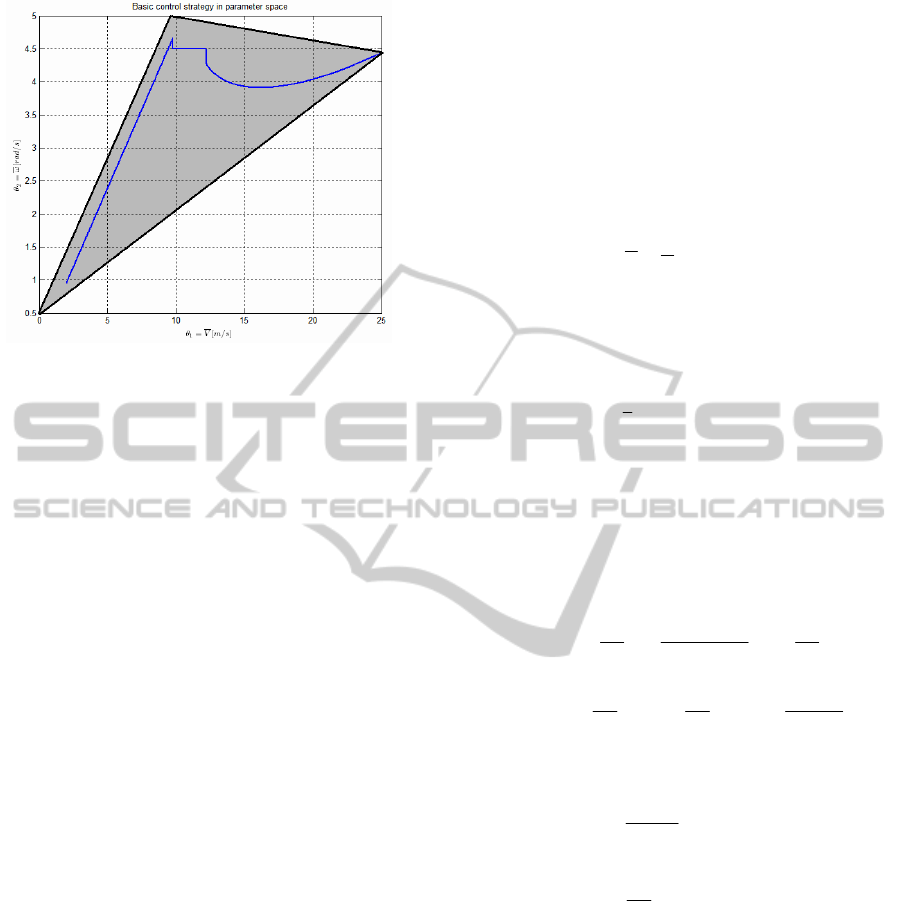
Figure 4: Parameter trajectory and polytope
Θ
.
in the parameter space
θ
. Hence, the controller
setup and design involve the optimization of the
control strategy tracking. Also note that the
operating points have been covered with a convex
polytope of three vertices
{
}
1 2 3
Co , ,
v v v
Θ = θ θ θ
, (18)
with
(
)
(
)
(
)
1 2 3
0; 0.5 , 9; 5 , 25; 4.43 .
v v v
= = =θ θ θ
In this favorable situation, as discussed in
Section 2, the synthesis of the LPV controller is very
simple. In fact, due to the LMIs multi-convexity
properties, we only have to check the set of LMIs
(14) at the vertices of
Θ
; the controller is then
obtained as a linear combination of three LTI
controllers.
3.3 LPV Model of Hawts
In case of VS-FP wind turbines, there is only one
control action, applied to the electrical machine.
Hence, a reduced model of HAWT will be used,
which neglects the high-frequency dynamics, treated
as model uncertainty. Despite the simplicity, the
reduced model describes well the dominant system
dynamics at low frequencies, thus is suitable for
designing a robust self-scheduled
∞
H
controller.
As stated in section 2, an LPV model of the
nonlinear system can be obtained by linearization
around a set of equilibrium points. Although the
LPV model is known only for a finite set of
scheduled variables
θ
, it is well defined for all
(
)
,
∈ Θ × Θ
θ θ
&
%
.
After the order reduction and the linearization
around a set of equilibrium points, the dynamic
model of the HAWT is described by (Bianchi
et al.,
2007):
( )
(
)
(
)
ˆ
ˆ
ω
ˆ
ˆ
:
ˆ
ω
ˆ
ω
ˆ
Z
S
G
Z
G
V Z
V
T
V
T
+ +
=


 


 
 

 
 
 

 
 
x = A θ x B θ B
M θ
Cx + D
&
, (19)
where the state and parameter vectors are:
[ ]
[ ]
ω
ˆ
ˆ ˆ
θ ω ω
T
T
S R G
V=
=
θ
x
. (20)
In this formulation, the bars and the hats over the
variables means operating point (steady-state) value,
and small variations with respect to the operating
point, e.g.
(
)
(
)
(
)
ˆ
V t V t V t
= +
, respectively. The
model’s inputs are the turbulence
ˆ
V
, regarded as a
disturbance, and the control action
ω
Z
. The outputs
are the shaft torque
S
T
, the generator speed and
torque. The matrices of the model are:
( )
( )
( )
( )
0 1 1
;
0 0 ;
0 0 ;
0 0
0 0 1 ; 0 0 . (21)
0 0 0
R S
S S
R R R
S S S G
G G G
T
R
V
R
T
G
Z
G
S S S
G G
b b
k b
J J J
k b b b
J J J
k
J
b
J
k b b
b b
−
+
= − −
+
−
=
=
−
= =
−
 
 
 
 
 
 
 
 
 
 
 
 
 
 
   
   
   
   
   
θ
A θ
θ
B θ
B
C D
In order to have a full description of the model
(19), a mathematical characterization of the
coefficients
(
)
(
)
and
R R
b k
θ θ
is required. These
coefficients have been obtained by linearization of
the power and the thrust coefficients,
(
)
λ
P
C
and
(
)
λ
T
C
, which are usually available for a given
HAWT. Thus, we have:
Self-scheduledH∞ControlofaWindTurbine-ARealTimeImplementation
407

( )
(
)
( )
( )
1 2
3 4
,
,
R R
R R
b b
k
V a V a
k V a V a
ω ω
ω ω
≡ = +
≡ = +
θ
θ
. (22)
The remaining parameters from equations (19) to
(22) are defined in Appendix. Note that the LPV
model (19) is affine in the parameter
θ
. This
property will turn out to be very useful for an LPV
controller design.
To accomplish the aforementioned control
objectives, we need to develop a series of tasks such
as the selection of the control scheme and controlled
variables, and computation of the reference signals.
A control scheme typically used to implement VS-
FP control strategy is a common speed feedback
loop. The speed reference is defined according to the
basic control strategy, i.e.
(
)
ω ω
ref ref
V
=
is the
function depicted in (17). Thus, the graph of
(
)
ω
ref
V
has the same shape as the basic control
strategy, plotted in Figure 4.
Figure 5: The open-loop LPV plant.
The first step of the LPV controller design is to
state the control objectives in terms of the
minimization of induced
2
norm
−L
of certain input-
output operator
:
zw
→
T w z
. This entails the
selection of the input variable w, the disturbance, the
virtual output variable z (called performance output)
and some weighting functions. Recall that the first
objective is to follow the control strategy, i.e. to
minimize the error
ε ω ω
ref G
= −
, and the second
objective is to the HAWT from excessive dynamic
loads. Therefore, by tacking:
[
]
~ ~
ˆ
ˆ
: ω
ˆ
: ε
T
ref
T
S
V
T
=
=
 
 
w
z
(23)
the objectives are introduced into the problem. Thus,
the corresponding LPV plant of the HAWT is
sketched in Figure 5, where
and
t
W W
ε
are the
weighting functions (to be determined), and
(
)
M
θ
is the input-output operator of HAWT, defined in
(19). It is worth mentioning that the output
[ ]
ˆ
T
G
ε ω =y
and parameter vectors are
measurable, which is an important aspect for the
implementability of the controller.
Under these assumptions, the open-loop LPV
model can be characterized as in (8), that is:
( )
(
)
(
)
1 2
1 11
2 21
: = ⋅
 
   
 
   
 
   
   
 
   
 
x A
θ B θ B x
G
θ z C D 0 w
y C D 0 u
&
, (24)
where
(
)
A
θ
is the same as in expresion (21), and:
(
)
(
)
[
]
1 2
1 11
2 21
3 1
; ;
0 0
0
; ;
0
0
0 0 1 0 1
; .
0 0 1 0 0
V Z
t S t S t S
W W
W k W b W b
ε ε
×
= =
−
= =
−
−
= =
   
   
   
   
   
   
B θ B θ B B
C D
C D
0
(25)
3.4 Controller Synthesis and Results
The model described in (24) and (25) is affine in the
parameter
θ
, that is:
(
)
( )
0 1 1 2 2
1 1,0 1 1,1 2 1,2
θ θ
θ θ
= + +
= + +
A θ A A A
B
θ B B B
. (26)
Moreover, the time-varying parameter
θ
is valued
in the convex polytope
Θ
(18). Hence, based on the
theorem presented in Section 2, we devise the
following constructive approach to the LPV self-
scheduled
∞
H
controller synthesis:
• compute a matrix
0
>
P
and adequate LTI
controllers
(
)
vi
θ
K
at the vertices
vi
θ
of the
parameter polytope, solving the LMIs (14);
• define LPV controller
(
)
θ
K
as an interpolant
of the vertex controllers
(
)
vi
θ
K
, as in (15).
The interpolation is based on the position of
θ
in the polytope
Θ
, given by the decomposition
(16).
Note that, in this case, the decomposition problem
has an unique solution:
ICINCO2012-9thInternationalConferenceonInformaticsinControl,AutomationandRobotics
408

(
)
( )
( )
( )
1
1 2 3
2
3
1 1 1
1
k
v v v
k
k
k
t
t
t
t
α
α
α
=
 
 
 
 
 
 
 
 
 
 
 
θ θ θ
θ
. (27)
Om_g
`
V_mean
y
theta
u
LPV control l er
V
Om_z
Ts
T_g
Om_g
P_g
Lambda
theta
HAWT nonl inear model
kG
Dampi ng injection
V Om_ref
Control strategy
P_g
:
T_g
.
Ts
,
Lam
'
Figure 6: Speed control loop for VS operation.
The LMI problem has been solved using the
Matlab’s LMI solver. The function feasp (Robust
Control Toolbox) solves the feasibility problem
defined by the given LMIs constraints (14). The
algorithm reaches convergence within 16 steps, for a
γ 1.03
=
. For a real time implementation, this
solution is computed off-line. With these
specifications, we can formulate a real time
synthesis algorithm.
Algorithm (Real Time controller)
Input. Matrices
, , , ,
, , , , 1, 2, 3
K i K i K i K i
i =A B C D
;
1. For
0
k
≥
1.1. At time
k
t
, the scheduling variable
(
)
k k
t
=
θ θ
is measured and the coefficients
(
)
i k
t
α
satisfying (27) are computed ;
1.2. The LPV controller matrices are computed:
(
)
(
)
( ) ( )
, ,
, ,
3
1
α
K i K i
K K
K i K i
K K
i
i=
 
 
=
 
 
 
 
∑
A B
A θ B θ
C D
C θ D θ
Output. The control signal
ω
Z
u =
, obtained by
integration of (10).
Simulation Results and Discussion
The nonlinear model of the HAWT, presented in
(Tudor, 2011), is used in the following simulations.
The wind speed signal is modeled as a non-
stationary random process, split in two components,
(
)
(
)
(
)
ˆ
V t V t V t
= +
. The mean wind speed is the
low frequency component, describing the behavior
of the wind currents on a long term. The turbulent
component
ˆ
V
corresponds to fast variations (high
frequency). In this paper, the turbulence is modeled
as a unity intensity white noise process filtered by an
adaptive stable filter von Karman.
The implemented speed feedback loop is sketched
in Figure 6. Its external signal
θ
is the measured
scheduling variable.
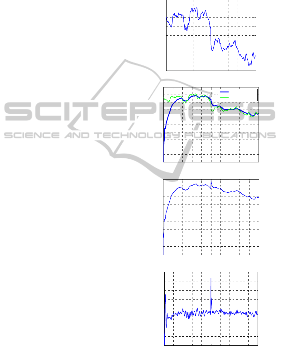
The step response of the closed-loop nonlinear
system is assessed first. Figure 7 shows the response
to a mean wind speed step in region I, from 9 m/s to
7 m/s, at t = 25 s. The control strategy is designed to
maximize the power conversion efficency, which is
equivalent to track the HAWT’s tip speed ratio
λ
at
its optimum value
8
opt
λ
=
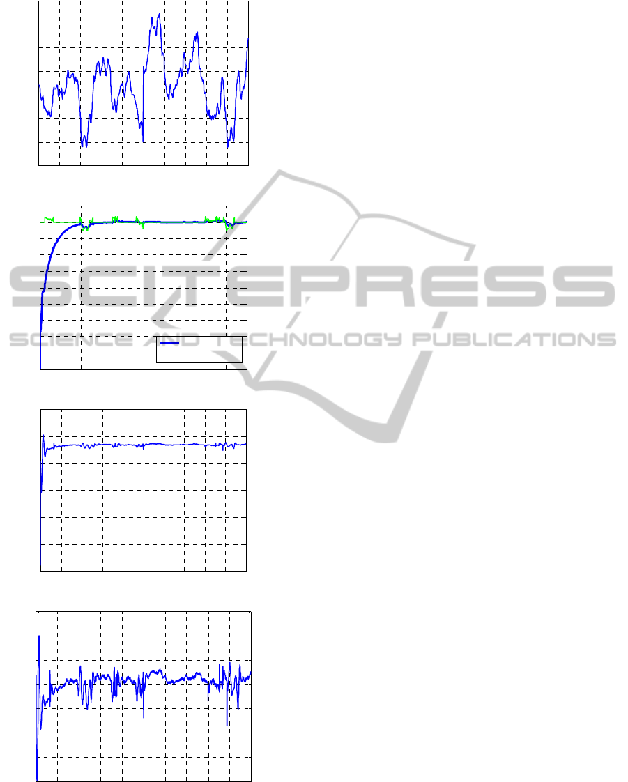
. In region II, large
oscillations are expected. The control objective is
therefore to limit the rotor speed at some well
chosen value (in this case,
nom
4.5
ω =
rad/s). This
situation is depicted in Figure 8; the mean wind
speed step is from 10.2 m/s to 11.8 m/s, at t = 25 s.
4 CONCLUSIONS
The simulations show that, in regions I and II, the
controller performances are quite good. More than
that, by analyzing the response of the closed-loop
system to a realistic wind profile, we can conclude
that the control objectives are fulfilled.
The real time algorithm, presented in section 3, is
efficient from the numerical point of view (the
number of arithmetic operations is quite small – the
convex decomposition problem consists in a 3x3
linear equation system; the computation of the
controller requires a low number of multiplications).
Thus, the LPV self-scheduled
∞
H
controller is
suitable for a real time implementation.
ACKNOWLEDGEMENTS:
The work has been founded by ERRIC project, FP -
7 - REGPOT - 2010 - 1, 264.207.
REFERENCES
Apkarian, P. and Adams, R. (1998). Advanced gain-
scheduling techniques for uncertain systems. IEEE
Transactions on Control Systems Technology 6 (1),
21–32.
Apkarian, P., Gahinet, P., Becker, G. (1995). Self-scheduled
Self-scheduledH∞ControlofaWindTurbine-ARealTimeImplementation
409

H∞ control of linear parameter-varying systems: a
design example. Automatica 31(9), 1251–1261.
Becker, G., Packard, A. (1994). Robust performance of
linear parametrically varying systems using
parametrically-dependent linear feedback. System &
Control Letters, 23 (205-215).
Bianchi, F. D., De Battista, H., Mantz, R. J. (2007). Wind
Turbine Control Systems. Principles, modelling and
Gain Scheduling Design. Springer-Verlag, London.
Burton, T., Sharpe, D., Jenkins, N., Bossanyi, E. (2001).
Wind Energy Handbook. John Wiley & Sons, LTD.
Jain, P. (2011). Wind Energy Engineering, McGraw Hill,
U.S.A.
Lescher, F. (2006). Commande LPV d’une eolienne a
vitesse variable pour l’optimisation energetique et la
reduction de la fatigue mecanique. Ph.D. thesis, Lille,
France.
Manwell, J. F., McGowan, J. G., Rogers, A. L. (2009).
Wind Energy Explained. Theory, design and
application. 2nd edition. John Wiley & Sons.
Packard, A. (1994). Gain scheduled via linear fractional
transformations. Systems and Control Letters 22(2),
79-92.
Pao, L. Y., Johnson, K. E. (2011). Control of Wind
Turbines-Approaches, Challenges and Recent
Developments, IEEE Control Systems Magazine, 4,
44-62.
Scherer, C.(1995). Mixed H2 / H∞ control, Trends in
Control: A European Perspective, Special
Contribution to the ECC’95 ed.
Scorletti, G., El Gahoui, L. (1998). Improved LMI
conditions for gain scheduling and related control
problems. International Journal of Robust and
Nonlinear Control 8(10), 845–877.
Tóth, R. (2010). Modeling and Identification of Linear
Parameter-Varying Systems. Springer - Verlag, Berlin.
Tudor, F. S. (2011). Modelling and control of a wind
turbine. Graduation thesis, Politehnica University of
Bucharest.
Wu, F. (2001). A generalized LPV system analysis and
control synthesis framework. International Journal of
Control 74(7), 745–759.
Wu, F., Yang, X., Packard, A., and Becker, G. (1996).
Induced L2-norm control for LPV systems with
bounded parameter variations rates. International
Journal of Nonlinear and Robust Control, 6(9-10),
983–998.
Zhou, K., Doyle, J., and Glover, K. (1996). Robust and
Optimal Control. Prentice-Hall, Englewood Cliffs,
USA.
APPENDIX
0 5 10 15 20 25 30 35 40 45 50
6
6.5
7
7.5
8
8.5
9
9.5
10
Wind speed
V (m/s)
Time (s)
0 5 10 15 20 25 30 35 40 45 50
0
0.5
1
1.5
2
2.5
3
3.5
4
4.5
5
Timp (s)
ω
G
,
ω
ref
(rad/s)
Speed regulation
Generator speed
ω
G
Speed reference
ω
ref
0 5 10 15 20 25 30 35 40 45 50
0
1
2
3
4
5
6
7
8
9
Tip speed ratio
Time (s)
λ
=
ω
R
R / V
0 5 10 15 20 25 30 35 40 45 50
1
1.5
2
2.5
3
3.5
4
4.5
5
x 10
5
Generated power
Time (s)
P
g
(W)
Figure 7: Closed-loop response in region I.
ICINCO2012-9thInternationalConferenceonInformaticsinControl,AutomationandRobotics
410

0 5 10 15 20 25 30 35 40 45 50
8.5
9
9.5
10
10.5
11
11.5
12
Wind speed
V (m/s)
Time (s)
0 5 10 15 20 25 30 35 40 45 50
0
0.5
1
1.5
2
2.5
3
3.5
4
4.5
5
Timp (s)
ω
G
,
ω
ref
(rad/s)
Speed regulation
Generator speed
ω
G
Speed reference
ω
ref
0 5 10 15 20 25 30 35 40 45 50
-4
-3
-2
-1
0
1
2
x 10
5
Generator torque
Time (s)
T
G
(Nm)
0 5 10 15 20 25 30 35 40 45 50
1.5
2
2.5
3
3.5
4
4.5
5
x 10
5
Generated power
Time (s)
P
g
(W)
Figure 8: Closed-loop response in region II.
Self-scheduledH∞ControlofaWindTurbine-ARealTimeImplementation
411