
Robust Arbitrary Reference Command Tracking
with Application to Hydraulic Actuators
M. G. Skarpetis, F. N. Koumboulis and A. S. Ntellis
Halkis Institute of Technology, Department of Automation, 34400, Psahna Evoias, Halkis, Greece
Keywords: Robust Control, Arbitrary Reference Command Tracking, Hydraulic Actuator.
Abstract: In this paper a robust tracking controller is proposed in order to track arbitrary reference signals in the
presence of same type disturbance signals. The robust tracking controller is based on the well known
Internal Model Principle appropriately modified with a Hurwitz invariability technique. The controller
parameters are computed using a finite step algorithm. Solvability conditions are derived. The proposed
controller is successfully applied to a hydraulic actuator uncertain model including uncertain parameters
arising from changes of the operating conditions and other physical reasons. Simulation results for all the
expected range of the actuator model uncertainties are presented indicating the satisfactory performance of
the robust controller in the presence of external disturbances.
1 INTRODUCTION
The problem of output tracking appears to be one of
the most popular control design problems (see (Chen,
1984), (Horowitz, 1963), (Dorf and Boshop, 2001),
(Goodwin et al., 2001), (Corless et al., 1984),
(Takaba, 1998); (Yaesh and Shaked, 1991) and the
reference therein). The problem of output tracking
for both non uncertain and uncertain systems (robust
tracking) is treated mainly using stabilizability
techniques, e.g. Dorf and Boshop, 2001; Corless et
al., 1984; Takaba, 1998. For robust tracking a variety
of approaches, to the most optimal or adaptive, has
been proposed in (Corless et al., 1984), (Takaba,
1998), (Yaesh and Shaked, 1991), (Skarpetis et al.,
2006a,b), and (Skarpetis et al., 2007).
The problem of robust tracking appears to be of
major interest in the design of controllers for
hydraulic actuators. This type of actuators is widely
used in many applications like manufacturing,
robotics, constructions and avionics. The dynamics
of fluid power are inherently uncertain. So, robust
control strategies are indispensible if one wishes to
guarantee safety and reliability of hydraulic actuators
(see Skarpetis et al., 2007; Karpenko and Shapehri,
2005; Koumboulis et al., 2006a and b; Koumboulis et
al., 1998; Kliffken, 1997; Kliffken and Heinrich,
2001; and the references therein). Robust asymptotic
tracking techniques like those in Skarpetis et al.,
2006a-b; Skarpetis et al., 2007 and robust PI-PID
design techniques like those in Koumboulis et al.,
2006a and b; Huang and Wang, 2000; Ho and
Huang, 2003; Musch and Steiner, 1995; Ge et al.,
2002; Toscano, 2005; Garcia et al., 2004;
Koumboulis, 2005; and Koumboulis, 1999; perform
satisfactory in many industrial hydraulic plants.
In this paper a robust tracking controller is
proposed in order to satisfy asymptotic command
following for arbitrary reference signals. The design
technique is based on the well known Internal Model
Principle (Goodwin et al., 2001), appropriately
extended using Hurwitz invariability for the
augmented system including the error dynamics. An
arbitrary reference model that produces desired
reference signals is used in the controller structure
and the overall closed loop robust stability is
guaranteed under sufficient conditions. The robust
tracking controller appears to guarantee satisfactory
performance under the influence of external
disturbance signals.
The present results are successfully applied to
control the position of a hydraulic actuator model
involving uncertain parameters arising from changes
of the operating conditions (temperature, pressure,
entrained air or water) as well as physical
uncertainties (loss in the effective area of the
actuator piston seal due to wear (Karpenko and
Shapehri, 2005)). Solvability conditions are
established. An analytic finite step algorithm for the
computation of the robust controller parameters is
94
G. Skarpetis M., N. Koumboulis F. and S. Ntellis A..
Robust Arbitrary Reference Command Tracking with Application to Hydraulic Actuators.
DOI: 10.5220/0004048600940102
In Proceedings of the 9th International Conference on Informatics in Control, Automation and Robotics (ICINCO-2012), pages 94-102
ISBN: 978-989-8565-21-1
Copyright
c
2012 SCITEPRESS (Science and Technology Publications, Lda.)

proposed. Following the algorithm, first, robust
stability regions are determined. Second, the
metaheuristic optimization algorithm proposed in
(Koumboulis and Tzamtzi, 2007) is applied, inside
these regions, to fulfil performance criteria. The
effectiveness of the controller is illustrated through
simulations for various values of the model
uncertain parameters. The present results appear to
be simple and easily applicable.
2 PRELIMINARY RESULTS
Consider the linear time-invariant SISO system with
non linear uncertain structure described by
() ()() ()() () ()
() () ()
xt Aqxt bqut dqwt
yt cqxt
=++
=
(1)
where
()
n
xt ∈ is the state vector, ()ut ∈ is the
input and
()yt ∈ is the output and ()wt ∈ is
external disturbance.
[
]
() ()
nn
Aq q
×
∈℘ ,
[
]
1
() ()
n
bq q
×
∈℘ ,
[
]
1
() ()
n
dq q
×
∈℘ and
[
]
1
() ()
n
cq q
×
∈℘ are function matrices depending
upon the uncertainty vector
1 l
qq q
⎡⎤
=∈
⎢⎥
⎣⎦
(
denotes the uncertain domain). The set ()q℘ is
the set of nonlinear functions of
q
. The uncertainties
1
,,
l
qq… do not depend upon the time. With regard
to the nonlinear structure of
(),Aq ()bq , ()dq and
()cq no limitation or specification is considered (i.e.
boundness, continuity).
Consider the case where the reference signal
()
r
yt is the output of a linear model described by
() () ; () ()
rrr rrr
xt Axt yt cxt==
(2)
where
()
r
yt∈ ,
1
()
r
r
xt
×
∈ and where
12 1
01 0 0
00 1 0
00 0 1
r
rr r
A
dd d d
−−
⎡⎤
⎢⎥
⎢⎥
⎢⎥
⎢⎥
⎢⎥
=
⎢⎥
⎢⎥
⎢⎥
⎢⎥
−− − −
⎢⎥
⎣⎦
,
10 0
r
c
⎡⎤
=
⎢⎥
⎣⎦
Consider the vector
,0r
x denoting arbitrary initial
conditions for system (2). Clearly, it holds that
() ( )
1
() () 0
r
rri
rir
i
yt dy t
−
=
+=
∑
(3)
The disturbance is assumed to be of the same type as
the reference signal, i.e.
() ( )
1
() () 0
r
rri
i
i
wt dw t
−
=
+=
∑
(4)
Define the tracking error
() () ()
r
tytytε =− (5)
Differentiating the error r-times, we get
() () ()
() ()
() () ()
() ( )
1
()
()
rrr
r
r
rri
ir
i
tcqxtyt
cqx t dy t
ε
−
=
=−=
=+
∑
(6)
or equivalently
()
() () ()
()
()
1
()
()
1
()
()
r
ri
r
i
i
r
ri
r
i
i
tdt
cqx t cq dx t
εε
−
=
−
=
+=
+
∑
∑
(7)
Define the variables
() ()
() ()
()
()
1
()
()
1
()
()
r
ri
r
i
i
r
ri
r
i
i
zt x t dx t
ut u t du t
−
=
−
=
=+
=+
∑
∑
(8)
According to (4), (7) and (8) the following
augmented system is defined:
()
() ()
()
d
xt Aqx bqut
dt
=+
(9)
() () () () ()
(1) ( 1)
T
r
xt t t t ztεε ε
−
⎡
⎤
=
⎢
⎥
⎣
⎦
() ()
()
1
()
0
,
0()
rr
r
nr
Aecq
Aq b q
Aq
bq
×
×
⎡
⎤
⎡⎤
⎢⎥
⎢⎥
==
⎢⎥
⎢⎥
⎢⎥
⎢
⎥
⎣⎦
⎣
⎦
,
(1)1
0
1
r
r
e
−×
⎡
⎤
⎢
⎥
=
⎢
⎥
⎢
⎥
⎣
⎦
.
Consider the static state feedback control law
() () () ()
12
ut fxt f t fztε==+
(10)
where
() () () ()
(1) ( 1)
T
r
ttt tεεε ε
−
⎡
⎤
=
⎢
⎥
⎣
⎦
.
The robust output command tracking is
formulated as follows (Chen, 1984; Goodwin,
Graebe and Salgado, 2001): the output of the
uncertain system (1) follows the output of the
reference system (2) while the tracking error (5)
RobustArbitraryReferenceCommandTrackingwithApplicationtoHydraulicActuators
95

decreases asymptotically to zero. This is satisfied
using a static state feedback control law of the form
(10) guaranteeing robust stability of the polynomial
() ()()
,, det
cl r n
psqf sI Aq bqf
+
⎡⎤
=−−
⎣⎦
(11)
The control law (10) can be expressed in terms of
the original systems using the differential equation:
()
()
() (1)
()
1,
11
()
()
2
1
() ()
()
rr
ri i
r
ii
ii
r
ri
r
i
i
ut du t f t
fx t dx t
ε
−−
==
−
=
+= +
⎛⎞
⎟
⎜
⎟
⎜
++
⎟
⎜
⎟
⎜
⎟
⎜
⎝⎠
∑∑
∑
(12)
where
1,
( 1,..., )
i
f
ir= are the elements of
1
f
. Eq.
(12) is realized in state space form as (see Figure 1):
2
() () (), () ()
() () ()
cccc cc
xt Axt b t t cxt
ut t fxt
ευ
υ
=+ =
=+
(13)
11,
21,1
1,1
10 0
01 0
,,
00 0
10 0
r
r
cc
r
c
df
df
Ab
df
c
−
⎡⎤⎡⎤
−
⎢⎥⎢⎥
⎢⎥⎢⎥
−
⎢⎥⎢⎥
==
⎢⎥⎢⎥
⎢⎥⎢⎥
⎢⎥⎢⎥
−
⎢⎥⎢⎥
⎣⎦⎣⎦
⎡⎤
=
⎢⎥
⎣⎦
,,
ccc
Abc
()wt
()
r
yt
()tε
()tυ
(),(), ()
()
Aq bq d q
cq
()xt
2
f
()ut
()yt
Figure 1: Closed loop structure.
3 SOLVABILITY CONDITIONS
The polynomial (11) can be rewritten as
()
() ()
,, det det ()
adj
cl r r n
nr
psqf sI A sI Aq
f
sI A q b q
+
⎡⎤⎡ ⎤
=− −
⎣⎦⎣ ⎦
⎡⎤
−−
⎣
⎦
(14)
Define:
() () ()
1
1
rn
aq a q a q
+
⎡⎤
=
⎢⎥
⎣⎦
(15)
where
()
i
aq
( 1,...,irn=+) are the coefficients
of the polynomial
[
]
[
]
det det ( )
rr n
sI A sI A q−−.
Also define the polynomial matrix
() ()
(
)
() ()
μ
+
=Ω =
⎡⎤
−
⎣
⎦
0
,[ ]
adj
qT
nr
Psq q s s
sI A q b q
(16)
where
()qnrμ ≤+ is the maximum degree of the
polynomial matrix
() ()
adj
nr
sI A q b q
+
⎡
⎤
−
⎣
⎦
and
() () ()
() () ()
0()
,1 ,
;
q
T
iiinr
qq q
qq q
μ
ωω
ωωω
+
⎡
⎤
Ω=
⎢⎥
⎣⎦
⎡
⎤
=
⎣
⎦
(17)
According to definitions (15) and (17) the
augmented closed loop characteristic polynomial
(14) can equivalently be expressed as follows:
()
0**
1
,, [ ] ()
nr
cl
T
psqf s sAq
f
+
⎡⎤
⎢⎥
=
⎢⎥
⎢⎥
⎣⎦
(18)
where
**
()
T
T
Aq a
⎡
⎤
=−Ω
⎢
⎥
⎣
⎦
%
%
,
()
() ()
()
()
0
nr nr q
qq
μ
+×+−
⎡
⎤
Ω= Ω
⎢
⎥
⎣
⎦
%
(19)
Based on the above definitions and the results in
(Wei and Barmish, 1989), (Koumboulis and
Skarpetis, 1996) and (Koumboulis and Skarpetis,
2000) the following theorem is presented.
Theorem 1. The problem of robust output command
tracking for the uncertain system (1) and for arbitrary
signals produced by the reference model (2), is
solvable, via the controller (13), if the following
conditions are satisfied
(i) The elements of
()
**
Aqare continuous functions
of
q for every
q ∈
(ii) There exists
()
1nr++ −row submatrix of
()
**
Aq, let
()
*
Aq which is positive antisymetric.
Proof: According to the definition of the problem
presented in Section 2, the problem of robust output
command tracking for the uncertain system (1) via
the controller (13) is solvable if the polynomial (14)
is robustly stable. According to the results in (Wei
and Barmish, 1989), (Koumboulis and Skarpetis,
1996) and (Koumboulis and Skarpetis, 2000) the
uncertain polynomial is Hurwitz invariant if
conditions (i) and (ii) of Theorem 1 are satisfied.
In the following theorem necessity is studied.
Theorem 2. For the problem of robust output
command tracking for the uncertain system (1) and
for arbitrary signals produced by the reference model
(2), via the controller (13), it is necessary for the
roots of the polynomial
[
]
()adj () ()
n
cq sI Aq bq− not
ICINCO2012-9thInternationalConferenceonInformaticsinControl,AutomationandRobotics
96

to be unstable roots of
det
rr
sI A
⎡⎤
−
⎣⎦
for every
q ∈
.
Proof: The polynomial (14) can be rewritten as
follows
()
() ()
() ()
1
2
,, det det ()
adj ( )adj
adj ( )det
cl r r n
rr n
nrr
psqf sI A sI Aq
fsIAcqsIAqbq
fsIAqbqsIAbq
⎡⎤⎡ ⎤
=− −+
⎣⎦⎣ ⎦
⎡⎤⎡ ⎤
−− − +
⎣⎦⎣ ⎦
⎡⎤⎡⎤
−− −
⎣⎦⎣⎦
From the above relation it is clear that if
()qσ ∈ is
a root of
[
]
()adj () ()
n
cq sI Aq bq− , being unstable
for at least one
q ∈ . Then its value for this q
must not be eigenvalue of
det
rr
sI A
⎡⎤
−
⎣⎦
.
The condition of Theorem 2 is related to the
uncontrollable part of the augmented system
() ()
(,)Aq b q
. This condition is useful in choosing
the model of the reference signal.
Remark 1. The class of the systems that satisfy
condition (ii) of Theorem 1, can be widen, if, instead
of
()
**
Aq the matrix
()
**
AqT is considered
where
T is an appropriate invertible and independent
from
q matrix.
For the definition of positive antisymetric
matrices see Wei and Barmish, 1989; Koumboulis
and Skarpetis, 1996; and Koumboulis and Skarpetis,
2000). An analytic algorithm for the computation of
an
f
preserving Hurwitz invariability can be found
in the aforementioned papers.
4 ROBUST CONTROL FOR
POSITION TRACKING OF A
HYDRAULIC ACTUATOR
4.1 Actuator Model
Consider a double acting servo valve and piston
actuator shown in Figure 2. The linearized
differential equations that describe the actuator –
valve dynamics can be formulated as follows
(Karpenko and Shapehri, 2005):
() ()
pp
xt tυ=
(20)
[]
1
() () () ()
pLpL
tAPtbtFt
m
υυ=−−
(21)
[]
4
() () () ()
LftpLp
Pt Kx t KPt A t
V
υ
β
υ
=−−
(22)
where
p
υ is the piston velocity,
p
x is the piston
position,
L
P is the hydraulic pressure across the
actuator piston,
L
F is the external load disturbance
and
x
υ
is the spool valve displacement. The
parameters
,,,Am bβ and V are: the piston surface
area, the mass of the load, the effective bulk modulus
of the hydraulic fluid, the viscous damping
coefficient and the total volume of hydraulic oil in
the piston chamber and the connecting lines,
respectively. The coefficients
f
K and
tp
K arise
from the linearization of the servo valve load flow
and the leakage flow.
v
x
p
x
b
q
A
L
P
m
p
υ
in
ν
Figure 2: Valve and piston schematic.
The valve displacement is usually produced by a
solenoid (electrohydraulic valve) actuated by the
input voltage
()
in
tν of the solenoid. The transfer
function of a solenoid can be approximated by the
servo valve spool position gain denoted by
v
k .
Using (20)-(22) the following linear system with
uncertain structure is derived in state space form:
00 0
() () () ( ) () ()
in L
xt A qxt B q t DF tν=+ +
(23)
0
() ()yt C xt= (24)
() () ()
()
T
ppL
xt t Pt
xt
υ
⎡
⎤
=
⎢
⎥
⎣
⎦
0
100C
⎡
⎤
=
⎢
⎥
⎣
⎦
0
112
01 0
() 0 / /
04/ 4/
Aq b m Am
qA V qq V
⎡
⎤
⎢
⎥
⎢
⎥
=−
⎢
⎥
⎢
⎥
⎢
⎥
−−
⎢
⎥
⎣
⎦
,
0
13
0
0
()
4/
Bq
qqk V
υ
⎡
⎤
⎢
⎥
⎢
⎥
=
⎢
⎥
⎢
⎥
⎢
⎥
⎣
⎦
,
0
0
1/
0
Dm
⎡⎤
⎢⎥
⎢⎥
=−
⎢⎥
⎢⎥
⎢⎥
⎣⎦
The parameter
1
q β= is an uncertain parameter
since the effective bulk modulus of the hydraulic
fluid changes due to temperature, pressure and
RobustArbitraryReferenceCommandTrackingwithApplicationtoHydraulicActuators
97

entrained air or water fluctuations. The parameter
2 tp
qK= changes due to migration of the system’s
operating point and the parameter
3
f
qK= changes
due to migration of the system operating point and to
loss in the effective area of the actuator piston seal,
due to wear (Karpenko and Shapehri, 2005). The
vector
123
qqqq
⎡⎤
=∈
⎢⎥
⎣⎦
is the uncertain
vector and
is the domain of uncertainty. The
nominal values of the system parameters are shown
in Table 1 and the expected range of variations of the
uncertain system parameters is shown in Table 2
(Karpenko and Shapehri, 2005).
Table 1: Nominal Values for the Hydraulic Actuator’s
Parameters.
Definition Nominal Values
V
volume of hydraulic
oil in the piston
chamber
33
468 / 100 m
A
piston surface area
22
633 / 1000 m
β
effective bulk modulus
6
689 10 Pa×
tp
K
total flow pressure
coefficient
3
0/mPas−
b
viscous damping
coefficient
1
1000Nm s
−
m
load mass
12Kg
k
υ
servo valve spool
position gain
3
0.0406 10 /mV
−
×
f
K
servo valve gain
2
1.02 / secm
Table 2: Expected Range of Variations of the Uncertain
Parameters.
Symbol
Minimum
Values
Nominal
Values
Maximum
Values
()Paβ
6
550 10×
6
689 10×
6
895 10×
3
tp
m
K
Pa s
⎛⎞
⎟
⎜
⎟
⎜
⎟
⎜
⎟
⎜
⎟
⎜
⎝⎠
0
0
11
9.5 10
−
×
2
sec
f
m
K
⎛⎞
⎟
⎜
⎟
⎜
⎟
⎟
⎜
⎝⎠
1.02
1.02
1.76
4.2 Robust Tracking Controller
In this subsection a robust tracking arbitrary
controller for asymptotic tracking of the piston
position will be designed. According to (2) the
reference output model is derived for
2r = to be:
,01
,0
,02
() (), () (),
r
rrrrrrr
r
x
xt Axt yt cxt x
x
⎡⎤
⎢⎥
===
⎢⎥
⎢⎥
⎣⎦
where
21
01
r
A
dd
⎡
⎤
⎢
⎥
=
⎢
⎥
−−
⎢
⎥
⎣
⎦
and 10
r
c
⎡⎤
=
⎢⎥
⎣⎦
.
According to definitions of Section 2 the
following augmented system is introduced
()
() ()
()
d
xt Aqx bqut
dt
=+
where
() ()
()
() ()
1
T
xt t t ztεε
⎡
⎤
=
⎢
⎥
⎣
⎦
()
21
112
010 0 0
10 0
000 1 0
000 / /
0004/ 4/
dd
Aq
bm Am
qA V qq V
⎡
⎤
⎢
⎥
⎢
⎥
−−
⎢
⎥
⎢
⎥
⎢
⎥
=
⎢
⎥
⎢
⎥
−
⎢
⎥
⎢
⎥
−−
⎢
⎥
⎣
⎦
,
()
13
0
0
0
0
4/
bq
qqk V
υ
⎡
⎤
⎢
⎥
⎢
⎥
⎢
⎥
⎢
⎥
=
⎢
⎥
⎢
⎥
⎢
⎥
⎢
⎥
⎢
⎥
⎢
⎥
⎣
⎦
.
Apply the static state feedback law: ufx=
with
11 12 21 22 23
f
fffff
⎡
⎤
=
⎢
⎥
⎣
⎦
. The aforementioned
controller can be produced by the original input
signal
()ut using the following state space form:
() () (), () ()
cccc cc
xt Axt bet t cxtυ=+ =
where
11,2
21,1
0
,,10
0
cc
df
Ac b c
df
−
⎡
⎤⎡⎤
⎡⎤
⎢⎥⎢⎥
===
⎢⎥
⎢⎥⎢⎥
⎣⎦
−
⎢
⎥⎢⎥
⎣
⎦⎣⎦
and
2
() () ()ut t fxtυ=+ where
2212223
f
fff
⎡⎤
=
⎢⎥
⎣⎦
.
The augmented system closed loop characteristic
uncertain polynomial is:
()
() ()
() () ()
543
12 0 1
21
234
,,, , ,
,,,
cl
psqqf s qfs qfs
qf s qf s qf
γγ
γγγ
=+ + +
++
(25)
ICINCO2012-9thInternationalConferenceonInformaticsinControl,AutomationandRobotics
98

where
()
12 23 3
10
4
,
()
u
mq q f k q bV
dq
mV
f
γ
−+
+=
,
()
22 1 3
12 23 3 1 12 2
2
11
33
12
1
(4
4( )4 (
,4
)
)
u
uu
Af k q q
mV
bq q f k q d mq q f k q
qf A
bd V d mV
qγ −+
−+ −+
+
=
,
()
2
2112112213
212 23 3
11 2 23 3 2
1
,(44()
4( )
(4 ( ) ))
u
u
u
qf Adq Af df kqq
mV
dmq q f kq
bdqq fkq dV
γ =−+
+−
+−+
,
()
3122233
2
2121212223
1
,(4(( )
()))
u
u
qf q bd q f kq
mV
Ad Af df d f k q
γ =−+
+− + +
,
()
1
4
122113
4(
,
)
u
Af df kq
qf
q
mV
γ =
+
−
.
According to (15) and (17) define
()
0123
10aq a a a a
⎡⎤
=
⎢⎥
⎣⎦
(26)
12
01
4bqq
d
m
a
V
++=
,
2
11211212
1
444bq q d mq q bd V d mV
m
a
V
Aq ++ ++
=
2
11 112 2 1
2
22
44 4Adq bdqq dmqq bdV
m
a
V
=
++ +
,
22
3
2
1
4( )dq A bq
mV
a
+
=
()
25
34 35
43 44 45
52 53 54 55
61 63
00000
0000
000
00
0
000
T
q
ω
ωω
ωωω
ωωωω
ωω
⎡⎤
⎢⎥
⎢⎥
⎢⎥
⎢⎥
⎢⎥
⎡⎤
⎢⎥
−Ω =
⎣⎦
⎢⎥
⎢⎥
⎢⎥
⎢⎥
⎢⎥
⎢⎥
⎣⎦
(27)
where
61 52 43
13
34
4
u
Ak q q
mV
ωωωω−====
,
13
25
4
u
kqq
V
ω −=
,
4
3
53
11
4
4
u
Ad k q q
mV
ωω=−=
,
13
35
1
4( )
u
kb dmqq
mV
ω
+
=−
,
23
55
1
4
u
bd k q q
mV
ω −=
,
5
3
63
21
4
4
u
Ad k q q
mV
ωω=−=
,
12
45
13
4( )
u
kbd dmqq
mV
ω
+
−=
,
According aforementioned definitions the
augmented closed loop characteristic polynomial
(25) can equivalently be expressed as follows:
()
543210**
11 12 21 22 23
,, ()
1
cl
T
psqf s s s s s sAq
fffff
⎡
⎤
=
⎢⎥
⎣⎦
⎡⎤
⎢
⎥
⎣
⎦
(28)
where
**
()
TT
Aq a
⎡
⎤
=−Ω
⎢
⎥
⎣
⎦
(29)
Let
100000
00 0 0 0 1
00 0 0 10
00 0 10 0
00 10 0 0
010000
T
⎡
⎤
⎢
⎥
⎢
⎥
−
⎢
⎥
⎢
⎥
−
⎢
⎥
⎢
⎥
=
⎢
⎥
−
⎢
⎥
⎢
⎥
−
⎢
⎥
⎢
⎥
−
⎢
⎥
⎣
⎦
Choose the following
66×
row submatrix of
()
**
AqT,
()
21 22
31 32 33
*
41 42 43 44
51 52 53 54 55
64 66
100000
0000
000
00
0
000 0
Aq
φφ
φφφ
φφφφ
φφφφφ
φφ
⎡
⎤
⎢
⎥
⎢
⎥
⎢
⎥
⎢
⎥
⎢
⎥
⎢
⎥
=
⎢
⎥
⎢
⎥
⎢
⎥
⎢
⎥
⎢
⎥
⎢
⎥
⎣
⎦
(30)
where
21 0
aφ =
,
()
31 1
qaφ =
,
41 2
aφ =
,
51 3
aφ =
,
22 25
φω=−
,
32 35
φω=−
,
42 45
φω=−
,
52 55
φω=−
,
33 34
φω−=
,
43 44
φω=−
,
53 54
φω=−
44 43
φω=−
,
54 53
φω−=
,
64 63
φω−=
,
55 52
φω=−
,
66 61
φω=−
.
Theorem 3. The problem of robust output
command tracking for the uncertain system (1) via
the controller (13) is always solvable.
Proof: Condition (i) can easily be verified. The
matrix
()
Aq
∗
is positive antisymetric. It can be
constructed using the five positive up augmentations
(
66
φ ,
55
φ ,
44
φ ,
33
φ and
22
φ are positive numbers
for all the values of the uncertainties):
() () () ()
() ()
1234
*
5
qqqq
qAq
Φ→Φ→Φ→Φ→
→Φ →
where
()
166
q φΦ=,
()
56
2
66
0
0
q
φ
φ
⎡⎤
⎢⎥
Φ=
⎢⎥
⎢⎥
⎣⎦
,
RobustArbitraryReferenceCommandTrackingwithApplicationtoHydraulicActuators
99

()
44
35455
64 66
00
0
0
q
φ
φφ
φφ
⎡⎤
⎢⎥
⎢⎥
Φ=
⎢⎥
⎢⎥
⎢⎥
⎢⎥
⎣⎦
,
()
33
43 44
4
53 54 55
64 66
000
00
0
00
q
φ
φφ
φφφ
φφ
⎡⎤
⎢⎥
⎢⎥
⎢⎥
Φ=
⎢⎥
⎢⎥
⎢⎥
⎢⎥
⎣⎦
,
()
22
32 33
42 43 44
512
52 53 54 55
64 66
0000
000
00
,
0
00 0
qq
φ
φφ
φφφ
φφφφ
φφ
⎡⎤
⎢⎥
⎢⎥
⎢⎥
⎢⎥
⎢⎥
Φ=
⎢⎥
⎢⎥
⎢⎥
⎢⎥
⎢⎥
⎣⎦
.
The vector
() ()
1
cq q=Φ
is a Hurwitz invariant
core since the associate polynomial of
()
cq
(
()
[
]
T
cq ) is positive Hurwitz invariant. Hence,
condition (ii) of Theorem 1 is satisfied. For reference
and disturbance signals of sinusoidal form, condition
(iii) of Theorem 1 is also satisfied.
5 COMPUTATION OF THE
CONTROLLER PARAMETERS
Using a reference input of the form
( ) 0.02 [0.2 ]
r
yt Sin t= (
12
0, 0.04dd==,
,01 ,02
0, 0.004
rr
xx==) the tracking controller will
be computed using the following algorithm
Step 1 (Construction of the augmentation
matrices): The core of
()
Aq
∗
is
() ()
1
cq q=Φ .
From
()
1
qΦ using five up positive augmentations
the matrix
() ()
6
qAq
∗
Φ= is constructed.
Let
1
1τ = .
Step 2 (Determination of the region of
1
0ε >
for which
()
21
1
T
q ε
⎡⎤
Φ
⎢⎥
⎣⎦
is positive Hurwitz
invariant): According to the form of the associated
polynomial it is observed that robust stability is
guaranteed
1
0ε∀>
. Let
21
1τε
⎡⎤
=
⎢⎥
⎣⎦
and choose
the stability region of
1
ε
to be :
[
]
1
0.25,0.55
ε
∈ .
Step 3 The polynomial
()
322
T
q ετ
⎡⎤
Φ
⎢⎥
⎣⎦
is
robustly stable
2
0ε∀>
. Let
321
1τεε
⎡⎤
=
⎢⎥
⎣⎦
and
choose the stability region of
2
ε
to be:
[
]
2
0.2,0.3
ε
∈ .
Step 4: The polynomial
()
433
T
q ετ
⎡⎤
Φ
⎢⎥
⎣⎦
is
positive Hurwitz invariant inside the selected
region
[
]
3
0.01, 0.015
ε
∈ .Let
4321
1τεεε
⎡⎤
=
⎢⎥
⎣⎦
.
Step 5 : The polynomial
()
544
T
q ετ
⎡⎤
Φ
⎢⎥
⎣⎦
is
positive Hurwitz invariant inside the region
99
4
610,710
ε
−−
⎡
⎤
∈× ×
⎣
⎦
.Let
54321
1τεεεε
⎡⎤
=
⎢⎥
⎣⎦
.
Step 6: The polynomial
()
655
T
q ετ
⎡⎤
Φ
⎢⎥
⎣⎦
is
positive Hurwitz invariant inside the selected
region
[
]
5
0.0006,0.0008
ε
∈ .
Step 7: Using a search algorithm in the stability
regions specified in steps 2-6 and for all values of
the uncertain parameters, the following values for
12345
,,,,εεεεε are derived:
1
0.5ε = ,
2
0.25ε = ,
3
0.012ε = ,
9
4
610ε
−
=×
and
5
0.0007ε = .
Step 8 (Derivation of the gain vector): The gain
vector
f
that robustly stabilizes the associated
polynomial of
()
**
AqT (
()
** T
AqTf
) is
54321
1f εεεεε
⎡
⎤
=
⎢
⎥
⎣
⎦
and consequently the
gain vector that robustly stabilizes the associate
polynomial of
()
**
Aq is
5 1234
1
T
T
Tf εεεεε
⎡
⎤
=−−−−−
⎢
⎥
⎣
⎦
or equivalently the vector
1234
5
55555
1
/1
T
T
Tf
εεεε
ε
εεεεε
⎡
⎤
⎢
⎥
=−−−−−
⎢
⎥
⎣
⎦
Finally using the above relation the respective values
from Step 7 of the algorithm and relation (28) the
controller parameters are computed to be
11 12
21 22
23
6
1428.57 714.286
357.143 17.1429
8.5714
,,
,,
3*1
0
ff
ff
f
−
−−
=− −
−
==
=
=
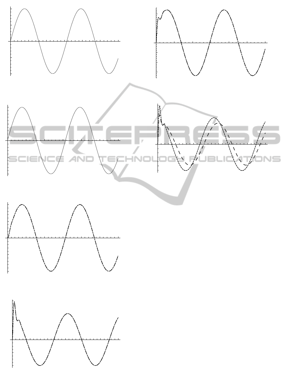
6 SIMULATION RESULTS
Using Table 1 and 2 and for a reference signal and
external disturbance as in Figures 3 and 4, the closed
loop performance is illustrated in Figures 5 – 7 and
the control signal is illustrated in Figure 8.
ICINCO2012-9thInternationalConferenceonInformaticsinControl,AutomationandRobotics
100
10 20 30 40 50 60
t
sec
0.02
0.01
0.01
0.02
Yr
t
Figure 3: Reference signal.
10 20 30 40 50 60
t
sec
10
5
5
10
F
L
t
N
Figure 4: External Disturbance.
10 20 30 40 50 60
t
sec
20
10
10
20
x
p
mm
Figure 5: The piston position.
10 20 30 40 50 60
t
sec
0.004
0.002
0.002
0.004
0.006
u
p
m
sec
Figure 6: The piston velocity.
10 20 30 40 50 60
t
sec
15
10
5
5
10
15
P
L
t
KPa
Figure 7: Hydraulic Pressure.
10 20 30 40 50 60
t
sec
0.05
0.05
V
in
t
V
Figure 8: Input voltage of the solenoid.
(Dotted line, Solid line, Dashed line is for the minimum, a
intermediary, and the maximum value of
q , respectively).
7 CONCLUSIONS
A Robust tracking controller has been designed for
arbitrary reference and disturbance signals.
Sufficient conditions have been derived and a finite
step algorithm has been proposed for fast and easy
computation of the controller parameters. The results
are successfully applied to a hydraulic actuator.
ACKNOWLEDGEMENΤS
The present work is supported by Archimedes III-
Strenghtening Research Groups In Technological
Education, NSRF 2007-2013.
REFERENCES
Chen, C. T., Linear System Theory and Design. Holt,
Rinehart and Winston, New York, 1984.
Corless, M. J., Leitmann, G., and Ryan, E. P., “Tracking
in the presence of bounded uncertainties,” presented at
RobustArbitraryReferenceCommandTrackingwithApplicationtoHydraulicActuators
101

the 4
th
Int. Conf. Control Theory, Cambridge, U.K.,
Sept, 1984.
Dorf, R. C., and Bishop, R. H., Modern Control Systems,
9
th
ed., prentice Hall, 2001.
Garcia, D., Karimi, A., Longchamp, R., “Robust PID
controller tuning with specification on modulus
margin”, Proceedings of the 2004 American Control
Conference, vol. 4, pp. 3297 – 3302.
Ge, M., Chiu, M.-S., Wang, Q.-G., “Robust PID controller
design via LMI approach”, Journal of Process
Control, vol.12, pp. 3-13, 2002.
Goodwin, G. C., Graebe, S. F., Salgado M.E., Control
System Design, Prentice Hall, 2001
Ho, F M.-T., Huang, S.-T. , “Robust PID controller design
for plants with structured and unstructured
uncertainty”, Proceedings of the 42nd IEEE
Conference on Decision and Control, 2003, vol. 1, pp.
780 – 785.
Horowitz, I. M., Synthesis Feedback Systems. New York
Academic, 1963.
Huang, Y. J., Wang, Y.-J. , “Robust PID tuning strategy
for uncertain plants based on the Kharitonov theorem”,
ISA Transactions, vol. 39, pp. 419-431, 2000.
Karpenko, M., Shapehri, N., “Fault – Tolerant control of a
servohydraulic positioning system with crossport
leakage”, IEEE Trans. on Contr. Syst. Technology,
Vol. 13, pp 155-161, 2005.
Kliffken, M. G., Heinrich, G. M., “A unified control
strategy for flight actuators”, Recent Advanced in
Aerospace Hydraulics, November 24-25, Toulouse,
France, 2001.
Kliffken, M. G., “Robust Sampled-Data Control of
Hydraulic Flight Control Actuators”, Proceedings of
the 5
th
Scandinavian International Conference on
Fluid Power, Linkoping, 1997.
Koumboulis, F. N., Industrial Control (in Greek), New
Technology Editions, 1999.
Koumboulis, F. N., “On the heuristic design of common
PI controllers for multi-model plants”, 10th IEEE
International Conference on Emerging Technologies
and Factory Automation, Catania, Italy, 2005, pp.
975-982.
Koumboulis, F. N., and Skarpetis, M. G., “Input -Output
decoupling for linear systems with non-linear
uncertain structure”, J. of the Franklin Institute, vol.
333(B), pp. 593-624, 1996.
Koumboulis, F. N., and Skarpetis, M. G., “Robust
Triangular Decoupling with Application to 4WS
Cars”, IEEE Transactions on Automatic Control, vol.
45, pp. 344-352, 2000.
Koumboulis, F. N., Skarpetis, M. G., Mertzios, B. G.,
“Robust Regional Stabilization of an Electropneumatic
Actuator”, IEEE Proceedings, Part D, Control Theory
and Applications, vol. 145, pp. 226-230, 1998.
Koumboulis, F. N., and Tzamtzi, M. P., A Metaheuristic
Approach for Controller Design of Multivariable
Processes, 12
th
IEEE Inter. Conf. on Emerging
Technologies and Factory Automation, Sept 25-28,
Patras, Greece, pp. 1429-1432, 2007.
Koumboulis, F. N., Skarpetis, M. G., Tzamtzi, M. P.,
“Robust PI Controllers for Command Following with
Application to an Electropneumatic Actuator”,
Proceedings of the 14th Mediterranean Conference on
Control Automation, Ancona, Italy, 2006.
Koumboulis, F. N., Skarpetis, M. G., Tzamtzi, M. P.,
“Robust PID Controller Design with Application to a
Flight Actuator”, Proceedings of the 32nd Annual
Conference of the IEEE Industrial Electronics Society
(IECON'06), pp. 4725-4730.
Musch, H. E., Steiner, M., “Robust PID control for an
industrial distillation column”, IEEE Control Systems
Magazine, vol. 15, pp. 46 – 55, 1995.
Skarpetis, M. G., F. N. Koumboulis and Ntellis, Α.,
“Robust Asymptotic Output Tracking for Four-Wheel-
Steering Vehicles”, IEEE International Conference on
Mechatronics, (ICM 2006), July 3-5, 2006, Budapest,
Hungary, pp. 488-492.
Skarpetis, M. G., Koumboulis, F. N., Ntellis, Α., “Robust
Tracking and Disturbance Attenuation Controllers for
Automatic Steering”, 14th IEEE Mediterranean
Conference on Control and Automation (MED’06),
June 28-30, 2006, Ancona, Italy.
Skarpetis, M. G., Koumboulis, Tzamtzi, M. P., “Robust
Control Techniques for Hydraulic Actuators ”, in
Proc. 15
th
MED Conf. on Control and Automation,
Athens, Greece 2007.
Takaba, K., “Robust preview tracking control for
polytopic uncertain systems”, in Proc. 37
th
IEEE Conf.
Decision Contr., Tampa, FL, 1998, pp. 1765-1770
Toscano, R., “A simple robust PI/PID controller design
via numerical optimization”, J. Process Control, vol.
15, pp. 81-88, 2005.
Yaesh , I. and Shaked, U., “Two degrees of freedom
H
∞
optimization of multivariale feedback systems”, IEEE
Transactions on Automatic Control, vol. 36, pp. 1272-
1276, 1991.
Wei, K, and Barmish, R., “Making a polynomial Hurwitz
invariant by choice of feedback gain”, Int. J. Contr.,
Vol 50, pp 1025-1038,1989.
ICINCO2012-9thInternationalConferenceonInformaticsinControl,AutomationandRobotics
102
