A Fast, Efficient Multi-Direct Forcing of Immersed Boundary

Method for Flow in Complex Geometry

Anyang Wei, Hui Zhao, Jin Jun and Jianren Fan

State Key Laboratory of Clean Energy Utilization, Zhejiang University, Hangzhou, P.R. China

Keywords: Immersed Boundary Method, Efficient, Fast, Multi-Direct Forcing.

Abstract: The Immersed Boundary method (IBM) has received wide attention from last decade, due to its promising

application to solve the fluid-solid interaction problems in large quantities of practical engineering areas.

This paper implemented IBM with Multi-Direct-Forcing (MDF), presenting the evaluation of momentum

forces on the body surface - interaction forces between fluid-solid. Grounded on the Multi-Direct-Forcing

method, we constructed a new system that could be efficiently and fast solved. Meanwhile, this proposed

algorithm is easy to code and implement parallelization. Besides, it can be extended to three-dimensional

simulation without much more extra efforts. Accuracy of the proposed MDF immersed boundary method

has been investigated, as well as some applications such as flow past the cylinder at a set of low Reynolds

numbers.

1 INTRODUCTION

The incompressible fluid flows involving complex

boundaries, which may be stationary or in motion,

are of practical and academic importance. These

problems can be solved by the traditional body-ﬁtted

numerical methods, in which governing equations

are discretized in a curvilinear coordinate system

that conforms to the boundaries, with re-meshing at

each time step. This procedure is not trivial and the

re-mesh computation is heavily cost. To solve the

complex geometrical fluid-interaction problem,

Peskin (Peskin 1972) proposed the Immersed

Boundary method in 1972, when he studied the flow

in heart valves based on the Cartesian grid. With

many structure grid properties retained, this method

gave the complex geometrical fluid-interaction prob-

lems an effective solution direction.

In the past two decades, we have seen the boom of

the Immersed Boundary Method. Several variants of

Immersed Boundary Method have appeared, like

Immersed Interface Method (Peskin 1972; Leveque

and Li 1994), Direct-Forcing Method (Uhlmann

2005) et al.. But all these methods, as the original

method proposed by Peskin, need an interpolation

between the immersed boundary Lagrangian and

Eulerian grid points. When this process is applied to

simple geometries or multiphase flows with a small

amount of particles, it is quantified. However, when

it comes to large quantities of particles or practical

geometries, it also costs a lot, though it is much

easier to implement than body-fitted numerical

method. These days, Ceniceros and Fisher

(Ceniceros and Fisher 2011) have applied the

treecode combined with FMM (Fast March Method)

to simulate large systems, but this method is not

trivial to implement. Wu and Shu et al.(Wu and Shu

2010) directly performed the fluid-interaction force,

deriving a linear system with the immersed bounda-

ry force density as variables. They deemed it was

easy to implement, but they only test two-

dimensional problems, however when it comes

across the three-dimensional systems or large quan-

tities of particles in multiphase flow simulation, that

linear system would be very huge, and the above

metioned FMM and treecode can be a good candi-

date.

Grounded on the work of Luo et al. (Luo, Wang

et al. 2007), Wu and Shu (Wu and Shu 2010), we

proposed another efficient fast immersed boundary

method based on the multi-direct-forcing immersed

boundary method. This paper is organized as fol-

lows. In section 2, firstly the governing equations for

the incompressible Navier–Stokes equations are

presented. Then immersed boundary method imple-

mented with multi-direct-forcing will be briefly

described. At the end of this section, we will propose

309

Wei A., Zhao H., Jun J. and Fan J..

A Fast, Efﬁcient Multi-Direct Forcing of Immersed Boundary Method for Flow in Complex Geometry.

DOI: 10.5220/0004049303090314

In Proceedings of the 2nd International Conference on Simulation and Modeling Methodologies, Technologies and Applications (SIMULTECH-2012),

pages 309-314

ISBN: 978-989-8565-20-4

 2012 SCITEPRESS (Science and Technology Publications, Lda.)

a fast and efficient algorithm based on above de-

scription. Several benchmark cases are simulated for

predicting the accuracy of the proposed MDF Im-

mersed Boundary method in Section 3. Finally, in

section 4, some concluding remarks will be drawn.

2 MATHEMATICS DESCRIPTION

2.1 Governing Equations of Fluid

The dimensionless governing equations for incom-

pressible flows in the computational domain



are:

t Re

 











      







u u u f

(1)

where

is the velocity of fluid;

is the pressure

and

is Reynolds number;

is the force density

of fluid-structure interaction. According to Luo et

al.(Luo, Wang et al. 2007) and Uhlmann (Uhlmann

2005), in multi-direct forcing method of IBM, the

force density

is calculated as

( ) ( ) ( )F d ,





  



f x X x X X

(2)

where

is the Eulerian coordinate; e.g. for two di-

mensional problems,

=( , ) ( 1 )

i i i

x x i , ,Nx

, where

is the number of Eulerian points. And the index

of coordinates are mapped into one-dimensional

index space from two dimensional computational

space for convenient as Wu & Shu (Wu and Shu

2010).

are Lagrangian coordinate and forcing

density on Lagrangian points, respectively. For two

dimensional problems, they can be denoted as

()

j j j

X ,XX

and

j j j

FF（ , ）F

( 1 )j , M

where

is the total number of Lagrangian points.

()



xX

is Dirac delta function.

2.2 Scheme of Multi-Direct-Forcing

In order to satisfy no-slip condition near the bounda-

ry, Lagrangian points coinciding with the boundary,

must be specified with a force

so as to the veloci-

ties at these points can be equal to velocities at

boundary. In the MDF method, the force can be

determined from Eq.(3)

t Re t



       



f u u u rhs

(3)

For the Lagrangian and Eulerian points, one can get

Eq.(4) and Eq.(5) respectively, according to Eq.(3),

( ) ( )

= ( ),

j j j

j j j j

ˆ ˆ















F X rhs X

U U U U

rhs X

(4)

( ) ( )

( ),

n 1 n

i i i

n 1 n

i i i i

ˆ ˆ













  

f x rhs x

u u u u

rhs x

(5)

where

and

are provisional velocities making the

second term zero.

()

( )=

j j j





U U X

(6)

The desired velocity is assumed that it can be

specified by known values, namely,

( )=

j j j



the boundary. Therefore, Eq.(4) can be reduced to

Eq.(6).

According to Uhlmann(Uhlmann 2005) and Wang

et al.(Wang, Fan et al. 2008), it is common to inter-

polate velocities from Eulerian points to Lagrangian

points with Dirac delta Function. There, this process

is directly written in the integral form; however, here,

we try to construct a fast algorithm, hence denote the

interpolation process as an operator A, namely,

( - )d d

M N N

ˆ ˆ











A u u x X x x

(7)

According to Eq.(7), we can get

Au U

. Then

force density on the immersed boundary

()

can

be directly evaluated. Once this force is calculated,

we can obtain the force density of Eulerian grid

points from the spreading process of

()

, that is

interpolating force on the immersed boundary back

to Eulerian grid.

As the same, we denote this spreading process as

an operator

NM

. So we have

N M M 1



f H F

(8)

Finally, we can get the velocities at the new time

step, namely





  u u f

(9)

However, after completing these two processes,

we may find actually the latest fluid field is not

completely satisfying the no-slip condition near the

immersed boundary, therefore MDF with the latest

fluid field redo the above two processes until the no-

slip boundary condition is achieved iteratively,

which is expressed in mathematical form as follows:

k 1 k k





  u u f

(10)

SIMULTECH 2012 - 2nd International Conference on Simulation and Modeling Methodologies, Technologies and

Applications

310

2.3 Fast Algorithm

In the work of Luo et al.(Luo, Wang et al. 2007), at

least twenty iterations are needed to achieve the no-

slip boundary condition. When it comes to solve the

large complex geometries or a number of particles in

fully resolved direct numerical simulation, algo-

rithms with twenty iterations are too cost. Here,

based on the previous work, we take a forward step

to obtain the no-slip boundary condition with much

less iterations.

So, we write the expansion of Eq.(10), and then it

gives

k 1 k k

k d k





  

  

u u HF

u HU HAu

(11)

From the above equation, it is not difficult to ob-

serve that as the iteration continues until

k 1 k

uu

the solution of this system converges. That means

HU HAu

(12)

Since

is known, the problem can be converted

into solving a linear system of

satisfying the

Eq.(12). To solve the above system, we need to

analyse the characteristics of the coefficient matrix

(denoting as

), so we can write down the

entries of this matrix

ij ik kj

q h a .





(13)

denotes the kth Lagrangian point spreading to the

ith Eulerian grid point;

denotes the jth Eulerian

point interpolating to kth Lagrangian point. Due to

the summation over all the Lagrangian points, so we

have

ij ji

qq

, this matrix is symmetrical, positive,

sparse, with many zero entries due to the cut off

effect of Dirac delta function. Here we apply the

steepest descent method to solve this system.

Here we define

as the residual of kth iteration of

system (12)

k k d

.r HAu HU

(14)

With we only need to evaluate the above defined

residual and an extra multiplication of matrix

with

vector

as well









r Qr

(15)

Finally, we can get the iteration formula as fol-

lows:

( ).

k 1 k k d



   u u HAu HU

(16)

3 NUMERICAL VALIDATION

To validate the accuracy of the algorithm proposed

above, we take the Taylor-Green vortices problem as

validation, which has an analytical solution. Then

uniform cross flows passed a single cylinder with

different Reynolds number are simulated. Drag coef-

ficients, lift coefficients and the Strouhal number of

vortex shedding are compared with previous results.

3.1 Taylor-Green Vortices

In order to validate the modified multi-direct-forcing

of Immersed Boundary method, two-dimensional

decaying vortices with analytical solution is studied.

Computational domain

[-1.5,1.5] [-1.5,1.5]





with a radius unity circular embedded in it is simu-

lated. The flow parameter

equals 100, the time

step



as Uhlmann (Uhlmann 2005) is 0.001, grid

size

is 1/64. The initial fluid fields and the bound-

ary conditions are both given according to the ana-

lytical solution. The numerical details of fluid solver

can be referred to Wang et al.(Wang, Fan et al.

2008).

The

2,uv

norm (Luo, Wang et al. 2007) is defined

as Eq.(17), where (

)is the desired veloci-

ties,and (

) is evaluated velocities on the kth

Lagrangian point,

[( - ) +( - ) ]

k d 2 k d 2

2,uv

u u v v





(17)

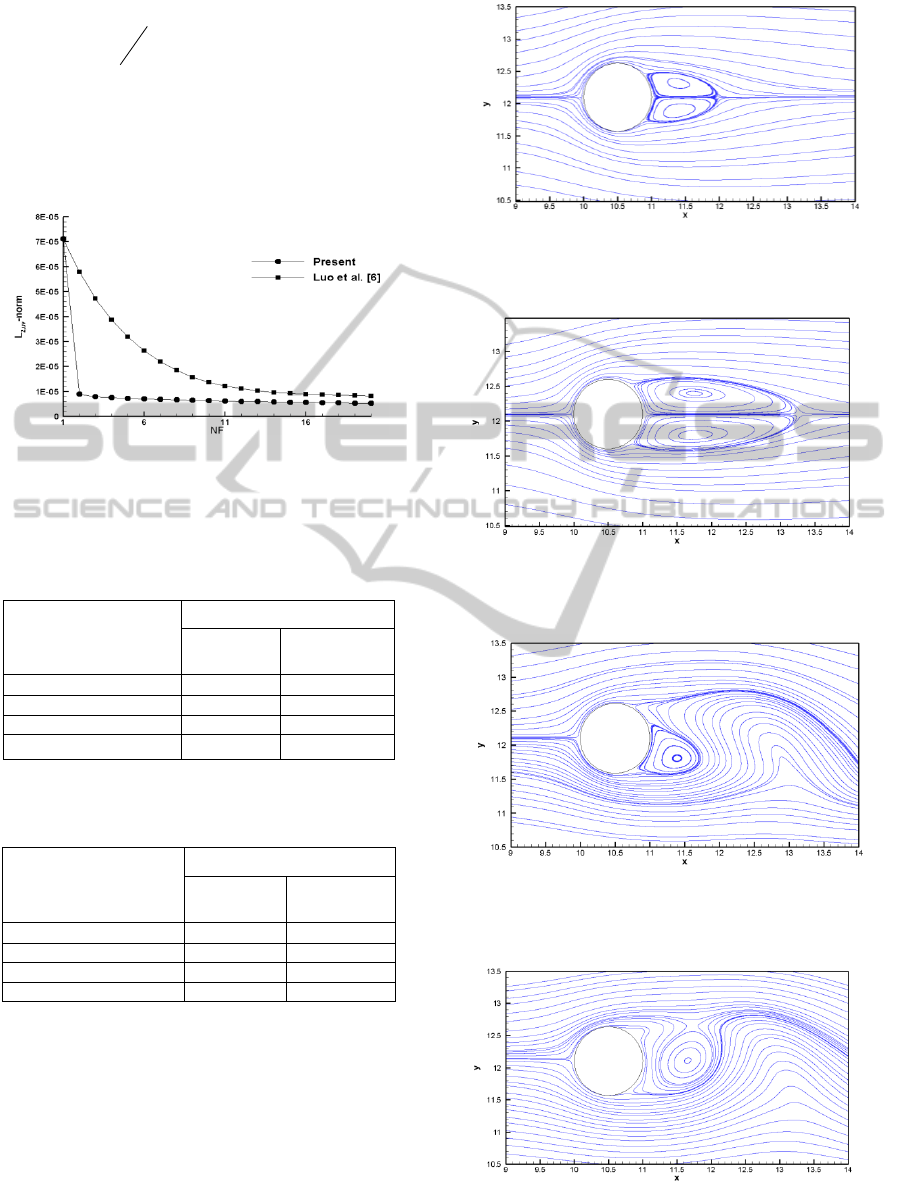
Figure 1 shows the fast convergence of present

modified multi-direct-forcing compared with the

previous Luo et al.(Luo, Wang et al. 2007), only

several iterations are needed to achieve the high

accuracy, which is much less than previous one.

Based on this, we choose to iterate 5 times for the all

latter simulation as default.

3.2 Flow Past Over a Cylinder

Flows past over a circular cylinder has been exten-

sively studied for verifying the algorithms of Im-

mersed Boundary Method. In this study, we place a

cylinder with diameter

0.6D 

at the location

(10.5D, 12.1D) in the domain

[0,35D] [0,24D]





At the inflow, we give a uniform free-stream veloci-

= (1, 0); at the

x= 24D

, we apply the convec-

tive out flow condition as Uhlmann (Uhlmann

2005). The ratio of

A Fast, Efficient Multi-Direct Forcing of Immersed Boundary Method for Flow in Complex Geometry

311

cylinder diameter to grid size is 30, and the Reynolds

number









in our simulation equals to 20,

40, 80, 100, and 200, respectively. And

0.001t





time step is used. Here, in present study, drag and

lift coefﬁcients and Strouhal number will be calcu-

lated for making a comparison with other numerical

and experimental results.

Figure 1: Correlation between the

2,uv

norm and the times

of multi-direct-forcing to show the fast convergence as

compared with the previous non-modified algorithm.

Table 1: Comparison of drag coefficient C

and recircula-

tion length

of Re=20.

Authors

Re=20

(Tritton 1959)

2.22



(Lima et al. 2003)

2.04

1.04

(Luo, Wang et al. 2007)

2.195

0.97

Present

2.146

0.97

Table 2: Comparison of drag coefficient C

and

recirculation length

of Re=40.

Authors

Re=40

(Tritton 1959)

1.48



(Lima et al. 2003)

1.54

2.55

(Luo, Wang et al. 2007)

1.62

2.35

Present

1.567

2.227

From the case

20Re 

and

40Re 

, it can be seen

from the streamline vector Figure 2 and Figure 3, the

wake behind the cylinder seems to be symmetric and

steady, which are in good agreement with the well-

established results. Table 1 shows that the drag co-

effcients and length of the recirculation zone

agreeing quite well with published results by

(Tritton 1959; Lima E Silva, Silveira-Neto et al.

2003; Luo, Wang et al., 2007).

Figure 2: The predicted results in the near wake of the

investigated circular cylinder at T = 200, streamline con-

tours, Re = 20.

Figure 3: The predicted results in the near wake of the

investigated circular cylinder at T = 200, streamline con-

tours, Re = 40.

Figure 4: The predicted results in the near wake of the

investigated circular cylinder at T = 200, streamline con-

tours, Re = 100.

Figure 5: The predicted results in the near wake of the

investigated circular cylinder at T = 200, streamline con-

tours, Re = 200.

SIMULTECH 2012 - 2nd International Conference on Simulation and Modeling Methodologies, Technologies and

Applications

312

The cylinder wake becomes unstable observed as

47Re 

. This is indeed what we predict from the

simulation carried out at Re = 100 and 200. Figure 4

and Figure 5 plots the streamline vector T = 200 for

Re = 100 and 200, respectively. As predicted, the

vortex shedding phenomenon is presented; hence the

modified multi-direct-forcing method can predict the

unsteady fluid flow in the complex geometries.

Table 3: Comparison of the predicted drag coefﬁcients, lift

coefﬁcients with other numerical results performed at Re =

100 and 200.

Authors

Re=100

(Clift 1978)

1.24



(Stålberg, Bruger et al.

2006)

1.32 ± 0.009

±0.33

(Chiu, Sheu et al. 2008)

1.34 ± 0.011

±0.32

(Calhoun 2002)

1.35 ± 0.014

±0.30

(Chiu, Lin et al. 2010)

1.35 ± 0.012

±0.3

Present

1.3140.009

0.32

Table 4: Comparison of the predicted drag coefﬁcients, lift

coefﬁcients with other numerical results performed at Re =

100 and 200.

Authors

Re=200

(Clift 1978)

1.16



(Stålberg, Bruger et al.

2006)



(Chiu, Sheu et al. 2008)

1.36 ± 0.048

±0.64

(Calhoun 2002)

1.17 ± 0.058

±0.67

(Chiu, Lin et al. 2010)

1.37 ± 0.051

±0.71

Present

1.2790.043

0.658

Table 3 and Table 4 give the comparison of the

predicted drag coefﬁcients, lift coefﬁcients of pre-

sent algorithm with other established results in

(Calhoun 2002; Stålberg, Bruger et al. 2006) at Re =

100 and Re = 200. We can find that in our simula-

tion results, the drag coefficient is lower than any

others’, with exception of Stålberg et al.(Stålberg,

Bruger et al. 2006), but it is more closer to the ex-

perimental data of Clift et al. (Clift 1978). The lift

coefficients at these two cases, predict almost the

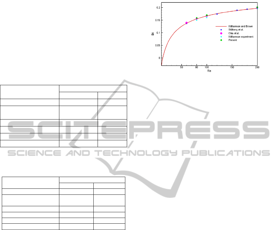
same with others. Meanwhile, we give the relation

of Strouhal number with Reynolds number, and

comparisons are made with the experimental corre-

lation formula and experimental data (Williamson

1996), as well as some other numerical results.

Thereby, the accuracy of present scheme can be

confirmed.

Figure 6: Strouhal number vs. Reynolds number.

4 CONCLUSIONS

In this paper, we proposed a novel fast and efficient

immersed boundary method implemented with mul-

ti-direct-forcing to evaluate the fluid-solid interac-

tions. The accuracy of the proposed multi-direct-

forcing immersed boundary method has been vali-

dated through the several benchmarks with only

several iterations, which are much less than previous

Multi-direct-forcing. However, we only test the two

dimensional applications. When it is applied to

complex three dimensional geometries, theoretically

it would not induce much more extra work, but the

problem whether the matrix calculation in three

dimensional cases will cause the extra cost so that it

induces inefficiency, should need much more care-

fully detailed numerical experiments in the future.

ACKNOWLEDGEMENTS

Financial support from the National Nature Science

of Foundation (No.51136006) of China is gratefully

acknowledged. We also thank Professor Kun Luo

for providing discussion and advice.

REFERENCES

Calhoun, D. (2002). A Cartesian grid method for solving

the two-dimensional streamfunction-vorticity

equations in irregular regions. Journal of

Computational Physics 176(2): 231-275.

Ceniceros, H. D. and J. E. Fisher (2011). A fast, robust,

and non-stiff Immersed Boundary Method. Journal of

Computational Physics 230(12): 5133-5153.

Chiu, P. H., R. K. Lin, et al. (2010). A differentially

interpolated direct forcing immersed boundary method

for predicting incompressible Navier–Stokes equations

A Fast, Efficient Multi-Direct Forcing of Immersed Boundary Method for Flow in Complex Geometry

313

in time-varying complex geometries. Journal of

Computational Physics 229(12): 4476-4500.

Chiu, P. H., T. W. H. Sheu, et al. (2008). An effective

explicit pressure gradient scheme implemented in the

two-level non-staggered grids for incompressible

Navier-Stokes equations. Journal of Computational

Physics 227(8): 4018-4037.

Clift, R., Grace, J., Weber, M. E. (1978). Bubbles, Drops,

and Particles, Academic Press,Inc.London Ltd.

Leveque, R. J. and Z. L. Li (1994). The Immersed

Interface Method For Elliptic-Equations with

Discontinuous Coefficients and Singular Sources.

Siam Journal on Numerical Analysis 31(4): 1019-1044.

Lima E Silva, A. L. F., A. Silveira-Neto, et al., 2003.

Numerical simulation of two-dimensional flows over a

circular cylinder using the immersed boundary method.

Journal of Computational Physics 189(2): 351-370.

Luo, K., Z. Wang, et al. (2007). Full-scale solutions to

particle-laden flows: Multidirect forcing and immersed

boundary method. Physical Review E 76(6): 066709.

Peskin, C. S. (1972). Flow patterns around heart valves -

numerical method. Journal of Computational Physics

10(2): 252-271.

Stålberg, E., A. Bruger, et al. (2006). High order accurate

solution of flow past a circular cylinder. Journal of

Scientific Computing 27(1-3): 431-441.

Tritton, D. J. (1959). Experiments On The Flow Past A

Circular Cylinder At Low Reynolds Numbers. Journal

of Fluid Mechanics 6(4): 547-567.

Uhlmann, M. (2005). An immersed boundary method with

direct forcing for the simulation of particulate flows.

Journal of Computational Physics 209(2): 448-476.

Wang, Z., J. Fan, et al. (2008). Combined multi-direct

forcing and immersed boundary method for simulating

flows with moving particles. International Journal of

Multiphase Flow 34(3): 283-302.

Williamson, C. H. K. (1996). Vortex dynamics in the

cylinder wake. Annual Review Of Fluid Mechanics

28(1): 477-539.

Williamson, C. H. K. and G. L. Brown (1998). A series in

1/√Re to represent the Strouhal–Reynolds number

relationship of the cylinder wake. Journal of Fluids

and Structures 12(8): 1073-1085.

Wu, J. and C. Shu (2010). An improved immersed

boundary-lattice Boltzmann method for simulating

three-dimensional incompressible flows. Journal Of

Computational Physics 229(13): 5022-5042.

SIMULTECH 2012 - 2nd International Conference on Simulation and Modeling Methodologies, Technologies and

Applications

314