
Replicator Dynamic Inspired Differential Evolution Algorithm for
Global Optimization
Shichen Liu, Yan Xiong, Qiwei Lu and Wenchao Huang
Department of Computer Science and Technology, University of Science and Technology of China,
Hefei, Anhui 230027, China
Keywords: Differential Evolution, Numerical Optimization, Parameter Adaptation, Self-adaptation, Replicator
Dynamic, Natural Computation.
Abstract: Differential Evolution (DE) has been shown to be a simple yet efficient evolutionary algorithm for solving
optimization problems in continuous search domain. However the performance of the DE algorithm, to a
great extent, depends on the selection of control parameters. In this paper, we propose a Replicator Dynamic
Inspired DE algorithm (RDIDE), in which replicator dynamic, a deterministic monotone game dynamic
generally used in evolutionary game theory, is introduced to the crossover operator. A new population is
generated for an applicable probability distribution of the value of Cr, with which the parameter is evolving
as the algorithm goes on and the evolution is rather succinct as well. Therefore, the end-users do not need to
find a suitable parameter combination and can solve their problems more simply with our algorithm.
Different from the rest of DE algorithms, by replicator dynamic, we obtain an advisable probability
distribution of the parameter instead of a certain value of the parameter. Experiment based on a suite of 10
bound-constrained numerical optimization problems demonstrates that our algorithm has highly competitive
performance with respect to several conventional DE and parameter adaptive DE variants. Statistics of the
experiment also show that our evolution of the parameter is rational and necessary.
1 INTRODUCTION
The evolutionary algorithms are heuristic search
algorithms which have been developed for over 50
years (Friedberg, 1958); (Box, 1957); (Holland,
1962); (Fogel, 1962). There are three main aspects
in EAs, i.e., genetic algorithms, evolutionary
programming and evolutionary strategies. They are
now generally used to solve optimization problems
in continuous search space. Differential Evolution
(DE) algorithm, proposed by Storn and Price, is one
of the state-of-the-art evolutionary algorithms (Storn
and Price, 1995). DE algorithm is a simple yet
efficient population-based stochastic method for
global optimization problems, and it has been
successfully applied to a whole host of engineering
problems such as aerodynamic design (Rogalsky et
al., 1999), digital filters design (Storn, 1996); (Storn,
2005), power system optimization
(Lakshminarasimman and Subramanian, 2008), etc.
Generally, just as other evolutionary algorithms,
there are three main operations in DE, i.e., mutation,
crossover and selection. In these operations three
crucial control parameters are required to be
specified. They are the population size NP, scale
factor F and the crossover rate Cr. These parameters
significantly affect the optimization performance of
the DE. In this regard, although the use of
evolutionary algorithms to solve problems of design
and optimization is varied, different end-users
confront the same problem that they have to find a
suitable parameter combination that matches the
evolutionary algorithms before actual design or
optimization can begin (Lobo and Goldberg, 2001);
(Harik and Lobo, 1999). Hence, it's reasonable and
necessary to turn parameters setting into a part of the
algorithm itself instead of leaving it as a problem to
the end-users.
In the past, on the choice of parameters of all
sorts of EAs, researchers always try to find a best
definite value for a parameter. To achieve this,
literature either uses a trial-and-error searching
process, or gets the parameter adapted or self-
adapted. However, in most cases, one cannot find a
best value for parameter configuration to optimize
the performance, and even whether there exists such
133
Liu S., Xiong Y., Lu Q. and huang W..
Replicator Dynamic Inspired Differential Evolution Algorithm for Global Optimization.
DOI: 10.5220/0004053401330143
In Proceedings of the 4th International Joint Conference on Computational Intelligence (ECTA-2012), pages 133-143
ISBN: 978-989-8565-33-4
Copyright
c
2012 SCITEPRESS (Science and Technology Publications, Lda.)

a best value is doubtful. More than one value of the
parameter may be appropriate: a value may win in a
run while a different value may perform better in
another run. Furthermore, there are also many cases
that some individuals of the population use a
parameter while the others use a different one obtain
better results than that the whole population uses a
definite parameter. So, unlike the previous studies,
which focus on finding a certain value for a
parameter, we focus on the probability distribution
of all possible or suitable values of the parameter, a
definite value is just a special form of the
distribution.
Based on the above observation, in this paper, we
propose a Replicator Dynamic Inspired DE
algorithm (RDIDE), in which crossover rate Cr is
configured using replicator dynamic, a deterministic
monotone game dynamic generally used in
evolutionary game theory. Since the probability
distribution of the crossover rate Cr is self-adapted
in our algorithm, the end-users can be able to simply
run the algorithm as a black-box without
consideration of the parameters, which may greatly
improve the working efficiency of the end-users.
To sum up, this paper makes the following
contributions:
We propose a new self-adaptive DE algorithm,
with which the users can solve their problems more
simply, with a higher success rate and a quicker
convergence speed.
Replicator dynamic is introduced to the
parameter setting of the DE algorithm. We no more
discuss about a proper parameter, but about an
advisable probability distribution of the parameter.
In the dynamic of the distribution, we design a
new mechanism for believable success rate based on
principle of statistics.
The remainder of this paper is organized as follows.
In section 2, the conventional DE is reviewed.
Section 3 describes the proposed RDIDE and the use
of replicator dynamic. A suite of 10 bound-
constrained numerical optimization problems is set
to evaluate the performance of the algorithm in
section 4. Finally, section 5 summarizes the main
conclusions arising from this work.
2 DIFFERENTIAL EVOLUTION
ALGORITHM
Without loss of generality, in this paper, DE is
aiming to minimize an objective function. Let S be
the search space of the optimization problem,
D
RS
. The population of DE includes NP individuals and
each of them is a D-dimensional solution particle. At
any certain generation G, the individuals are of the
form
NP,1,2,i ,
321
)
G
i,D
x
G
i,
,x
G
i,
,x
G
i,
(x
G
i
X
,
S
G
i
X
,
where i indicates the index of the particle. The
particles develop from one generation to another
constraint by the search space. At each generation,
every particle goes through the operations of
mutation, crossover and selection, and a trial particle
will be generated for each target particle. The
evolution processes as follows.
2.1 Initialization
DE algorithm starts with an initial population
}XX,X,X{
NP
00
3
0
2
0
1
, these particles are expected to be
initialized filling the entire search space as much as
possible. For this purpose, generally, the initial
population is generated within the boundary
constraints at random
D,1,2,j ,10
0
)X(X),N(XX
L
j
U
j
L
ji,j
(1)
where
L
j
X
and
U
j
X
are the lower and upper boundary
of j-th component respectively, and
),N( 10
denotes
a uniformly distributed random value within the
range [0, 1].
2.2 Mutation
A mutant vector
)y,y,y(yY
G
i,D
G
i,
G
i,
G
i,
G
i
,
321
is generated
for every associated target vector
G
i
X
in this
operation at each generation G. Several mutation
methods could be used to generate
G
i
Y
, and a
conventional one is like this:
NP,2, 1,i,
321
)XX(FXY
G
i
r
G
i
r
G
i
r
G
i
,
(2)
where index
iii
randrr
321
,
are random integers from
the range [1, NP], mutually different, and each is
different from the base index i. F is a scaling factor
for differential vectors.
2.3 Crossover
Crossover operation comes after mutation. The trial
vector
),,,,(
,3,2,1,
G
Di
G
i
G
i
G
i
G
i
uuuuU
is generated from the
combination of its parent and mutant vector:
otherwise,x
)jor(jCR)[0,1)if(Uniform,y
G
ji,
randji,
G
ji,
,
G
ji
u
(3)
IJCCI2012-InternationalJointConferenceonComputationalIntelligence
134

where
rand
j
is a random index chosen from [1, D] to
ensure at least one component is different from
G
i
U
and
G
i
X
, and the parameter Cr is within the range [0,
1], indicating the crossover rate of the generation. If
any component of the trial vectors is beyond the
search space, they will be reinitialized randomly and
uniformly within the search space.
2.4 Selection
In this phase, we determine which vector is going
into the next generation and which should be
deleted. The procedure is done following rule for the
function minimization:
otherwiseU
UfXfifX
X
G
i
G
i
G
i
G
i
G
i
,
))()((,
1
(4)
Every trial vector is only compared with its target
vector, and the one with better fitness is kept. Hence,
all the individuals of the next generation are going to
get better or remain the same, thus the whole
population evolves.
3 REPLICATOR DYNAMIC
INSPIRED DE ALGORITHM
Being a crucial factor of the DE algorithm, control
parameters selection determines the performance of
the algorithm directly. Hence, a good deal of
research on the parameters selection of DE has been
done. Storn (1995) suggested that F within the range
[0.5,1], Cr in [0.8,1] and NP = 5D or 10D. Gämperle
et al. (2002) suggested that NP be between 3D and
8D, F= 0.6, and Cr between [0.3,0.9]. At the same
time, several adaptive and self-adaptive mechanisms
have been proposed to dynamically change the value
of the parameters. Zaharie (2003) used a
multipopulation method for the parameter adaptation
(ADE). Omran et al. (2005) proposed a mechanism
to self-adapt the scaling factor F (SDE). Later on,
Brest et al. (2006) encoded F and Cr into individuals
and modulate them by two parameters. In the same
year, Teo (2006) proposed a DE algorithm with a
dynamic population sizing strategy based on self-
adaptation (DESAP). Lately, Qin et al. (2009)
proposed SaDE, in which both generation strategy
and the parameters are adapted.
In our paper, we focus on the adaptation of Cr
during the evolution, as Cr is an especially
significant parameter. The suitable choice of Cr can
lead to good result while an improper one may result
in the failure of the algorithm (Price et al., 2005).
3.1 Inspired by Replicator Dynamic
The main idea of this paper is to self-adapt the
probability distribution of the crossover rate, so that
the parameter could be more suitable to various
kinds of problems. At the same time, different
distributions of Cr may perform better at different
generations for a certain problem, so the distribution
of Cr is expected to be fit for every moment of the
evolution as well. To achieve this, a mechanism of
multiple evolutions is proposed: the first evolution
refers to DE algorithm itself, and the second one
means that the probability distribution of Cr value is
evolving independently with the idea of evolutionary
game theory.
We build a candidate set (CRSet), containing
several possible values of Cr. Whenever the
crossover operation is executed, each individual
choose one value from the set via a particular
probability distribution. The value of Cr is a real
number within the range [0, 1], and the set is
expected to cover the range uniformly. In our
proposal, we let
CRSet
,,,{
321
CRCRCR },
54
CRCR
,
where
i
CR
is set to (0.2×i-0.1). For each
i
CR
, a
i
P
is assigned to indicate the probability to choose it,
the distribution of
i
P
is
P
. At each generation,
every individual choose a Cr from the CRSet via the
distribution of
i
P
, and the distribution
P
is evolving
according to the fitness of each
i
CR
of the current
and previous generations with replicator dynamic.
Probability distribution to choose values for Cr is
very similar to mixed strategy equilibrium of a game
theory, and a definite value of Cr corresponds with a
pure strategy. Our attention is on the dynamically
changing of the distribution, thus a method of
evolutionary game theory is introduced. We assume
that a new population of plentiful individuals is
generated to seek a reasonable probability
distribution for
i
CR
with the idea of evolution. Any
individual in the population is called replicator,
choosing a certain value in the CRSet and passing its
choice to the descendants without modification. Let
tn
i
be the number of individuals choosing
i
CR
at
time point t, then the total population size is
tntN
ii
5
1
, and the proportion of individuals to
choose
i
CR
is
tNtntpcr
ii
/
. The population
state is the distribution of
tpcr
i
, i.e.,
,(
1
tpcrtP
cr
.
),,,
5432
tpcrtpcrtpcrtpcr
, Let
and
be the
ReplicatorDynamicInspiredDifferentialEvolutionAlgorithmforGlobalOptimization
135

background per capita birth and death rates in the
population. Then the rate of change of the number of
individuals choosing
i
CR
(
i
n
) and rate of change of
total population (
N
) can be described as follows:
iii
nCRfitnessn
)(
(5)
)(
)(
5
1
5
1
5
1
CRfitnessN
N
nCRfitness
NnnN
i
ii
i
i
i
i
(6)
where
5
1
)()(
i
ii
pcrCRfitnessCRfitness
is the
average fitness.
Since
tNtntpcr
ii
/
, we take derivative to
both sides:
iii
pcrNnrcpN
. So
iii
pcrCRfitnessCRfitnessrcp )()(
(7)
(7) gives the replicator dynamic that will be used to
adjust distribution of
i
pcr
, increasing rate of the
proportion of the individual choosing
i
CR
is
independent of the background per capita birth rate(
), death rate(
) and the size(
tN
) of the
population. In another word, the evolution of
cr
P
is
only dependent on the fitness of each Cr, which is
very simple to execute. We let the possibility of one
particle (an individual in DE) to choose
i
CR
equal
the proportion of individuals (in Cr evolution) to
choose
i
CR
, i.e.,
crii
PPpcrP
,
, to ensure that the
proportion of individuals in DE to choose different
Cr is approximate to
cr
P
.
)(
i
CRfitness
can be
indicated by the success rate of the trial vectors
generated by
i
Cr
i
CrT
and successfully entering the
next generation
i
CrW
. So, (7) changes into the form
below:
i
ii
CrT
CRSuccRateCRfitness
i
CrW
)()(
(8)
pcrCRSuccRateCRSuccRateP
ii
)()(
(9)
51,2i ,)()(
5
1
,,
i
ii
PCRSuccRateCRSuccRate
(10)
The distribution
P
changes by (8), (9) and (10)
succinctly, thus the evolution of Cr is achieved.
3.2 Design of Believable Success Rate
When we use the replicator dynamic for the
evolution of Cr, there is still a problem in (8), that if
the total quantity of individuals using
i
CR
is not
enough, the corresponding fitness is trustless.
So we have to determine the minimum of
i
CrT
to ensure the trustiness of
)(
i
CRfitness
with high
confidence level and narrow confidence interval.
From de Moivre–Laplace theorem, we learn that if
i
CrT
is big, approximately
1 0,N~
1 CRfitnessCRfitnessCrT
CRfitnessCrTCrW
where
1 0,N
denotes the standard normal
distribution and indexes are omitted. Thus we have:
1
1
2/2/
u
CRfitnessCRfitnessCrT
CRfitnessCrTCrW
uP
(11)
Equation can be transformed into another form:
1)( BCRfitnessAP
(12)
The solutions of the equation
2
2/
2
1
u
CRfitnessCRfitnessCrT
CRfitnessCrTCrW
are A and B:
2
/2
2
2
/2
/2
/2
2
ˆ
()
2
,
ˆˆ
() 1 ()
4
u
fitness CR
CrT
CrT
AB
CrT u
u
fitness CR fitness CR
u
CrT
CrT
(13)
where
CrTCrWCRssefitn /)(
ˆ
, denotes the value of
fitness that will be used in the algorithm,
2/
u
is a
corresponding constant to
in
1 0,N
, A takes
negative sign and B takes positive sign.
1
is the confidence level and
BA,
is the
confidence interval for
)(CRfitness
. Since
1)(
ˆ
0 CRssefitn
,
4/1)(
ˆ
1)(
ˆ
CRssefitnCRssefitn
. When we assume
4/1)(
ˆ
1)(
ˆ
CRssefitnCRssefitn
,
the width of
BA,
equals to
2
2/2/
/
uCrTu
. Let
05.0
and
2.0widththe
, we have
96.1
2/
u
and
the minimum of CrT is 93. This is to say, CrT must
be at least 93,
)(
ˆ
CRssefitn
is trusted.
However, CrT could not be big enough in one
generation, so two extra methods are introduced to
RDIDE. First we build memories to store the
numbers of individuals choosing
i
CR
and those
successfully entering the next generation within the
last M generations. With this method,
MGCrTCrWCrTCrWCRssefitn
G
MGg
g
i
G
MGg
g
iiii
11
//)(
ˆ
where G is the current generation, and respectively,
g
i
CrT
and
g
i
CrW
denote the number of vectors
IJCCI2012-InternationalJointConferenceonComputationalIntelligence
136

choosing
i
CR
in generation g and the number of
those successfully entering the next generation.
During the first M generations, we simply let the
value of
i
P
be 0.2 (i = 1, 2, 3, 4, 5), and add
g
i
CrT
and
g
i
CrW
to the memories. In the following
generations,
i
P
is dynamically changing with (9),
while
g
i
CrT
and
g
i
CrW
replace
Mg
i
CrT
and
Mg
i
CrW
.
Besides, we assign a constant (
min
P
) to constrain the
minimum of
i
P
, when
i
P
<
min
P
and
i
P
is going to
decrease, the value of
i
P
remains the same. The
expected value of CrT,
MPNPCrTE )(
. In this
paper,
)(CrTE
is expected to be equal or greater than
100 to ensure the trustiness of
)(CRfitness
, and we
achieve this by assuming a small P such as 0.1, and
NPPM //100
.
3.3 The Algorithmic Description
The algorithmic description of the RDIDE is
presented in Table 1.
Table 1: Algorithmic description of the RDIDE.
Step 1: Initialization
Set the generation counter G=0.
Initialize a population of NP individuals according to (1). Evaluate the
population. Store with best fitness as and its fitness .
Initialize the distribution of , , and establish two
memories, , (i=1 to M, j=1 to 5).
Step 2: Evolution
WHILE Termination Criterion is not satisfied
Step 2.1 renovate and
Replace and by and
Set ,
Step 2.2 Mutation, Crossover and Selection
FOR i=1 to NP
Choose a from CRSet due to
FOR j=1 to D
END FOR
WHILE the variable is outside the search region
Regenerate
END WHILE
Evaluate the trial vector.
IF
,
IF
END IF
ELSE
END IF
END FOR
Step 2.3 Dynamic Change of Distribution
IF G>M
ReplicatorDynamicInspiredDifferentialEvolutionAlgorithmforGlobalOptimization
137

Table 2: Benchmark functions.
Test problems
min
f
global optimum S
D
i
i
zF
1
2
1
0o
D
100,100
D
i
i
j
j
zF
11
2
2
0o
D
100,100
1
1
2
2
1
2
11003
D
i
iii
xxxF
0 (1,1,…,1)
D
100,100
1,04.014
11
2
NzF
D
i
i
j
j
0o
D
100,100
ez
D
z
D
F
D
i
i
D
i
i
202cos
1
exp
1
2.0exp205
11
2
0o
D
32,32
em
D
m
D
F
D
i
i
D
i
i
202cos
1
exp
1
2.0exp206
11
2
0o
D
32,32
D
i
D
i
ii
i
zz
F
1
1
2
1cos
4000
7
0o
D
500,500
D
i
D
i
ii
i
mm
F
1
1
2
1cos
4000
8
0o
D
500,500
D
i
ii
zzF
1
2
102cos109
0o
D
5,5
D
i
ii
mmF
1
2
102cos1010
0o
D
5,5
zMmoooooxz
D
,,,
,,2,1
;o: the shifted global optimum, M: orthogonal rotation matrix.
F6:cond(M)=1; F8:cond(M)=3; F10:cond(M)=2
4 EXPERIMENTS AND RESULTS
4.1 Test Problems and Experimental
Conditions
In this paper, in order to assure a fair comparison,
the experimental conditions, the parameters setting
and the benchmark problems are the same to SaDE.
10 benchmark problems (F1-F10) were set to
evaluate the performance of our algorithm. Six
functions (F1, F2, F4, F5, F7, F9) are shifted and
three (F6, F8, F10) are further rotated. Among these
functions, F1-F4 are unimodal functions and F5-F10
are multimodal functions. All the functions are listed
in Table 2.
In our experiment, RDIDE is compared with 5
conventional DE and 4 adaptive DE variants. In
order to ensure reliability, the statistics of the
experiment with these 9 DE algorithms are results
found in literature (Qin et al. 2009). The conditions
of the experiment are as follows:
1) Population size NP=50, Scaling factor F=0.5;
2) Dimension D=10/30 for all problems:
FEs=100 000 with 10-D problems,
FEs=300 000 with 30-D problems.
3) Parameters for RDIDE,
1.0,20
min
PM
.
4) Comparison DE, 5 conventional DE:
DE/rand/1(F=0.9,Cr=0.1),
DE/rand/1(F=0.9,Cr=0.9),
DE/rand/1(F=0.5,Cr=0.3),
DE/rand-to-best/1(F=0.5,Cr=0.3),
DE/rand-to-best/2(F=0.5,Cr=0.3).
4 adaptive DE variants:
SaDE, ADE, SDE, jDE.
5) All experiments were run 50 times,
independently.
4.2 Results and Analysis
1) In this section, we compare RDIDE with the 9
other DE. Two groups of comparison are conducted
to show the highly competitive performance of
RDIDE. In the first comparison, we concentrate on
the mean and standard deviation of the functions as
well as the success rates. The success rate refers to
the proportion that the success runs divided by the
total runs. The success of a run means that it results
in a value no worse than the pre-specified optimal
value, i.e.,
5
min
10
f
with the number of FEs less
than the pre-specified maximum number in this run.
In the second comparison, we focus on the average
number of function evaluations (NFE) required to
find the optima, as it’s a direct reflection of the
convergence speed. Table 3 and Table 4 report the
statistics of the first comparison, and Table 5 shows
the results of the second comparison. All best results
are typed in bold.
From the results of the first comparison, we can
IJCCI2012-InternationalJointConferenceonComputationalIntelligence
138

Table 3: Results for 10-D problems.
Algorithm
D=10
F1 F2 F3 F4
Mean Std SRate Mean Std SRate Mean Std SRate Mean Std SRate
CDE-1 0 0 100% 8.89E-01 4.96E-01 0% 9.01E-01 7.94E-01 0% 2.41E+01 1.28E+01 100%
CDE-2 4.95E-13 5..27E-13 100% 1.44E-05 1.13E-05 43% 7.11E-03 2.74E-02 0% 2.42E-04 1.38E-04 100%
CDE-3 0 0 100% 9.63E-09 5.99E-09 100% 1.76E+00 1.54E+00 0% 5.42E-06 4.44E-06 83%
CDE-4 0 0 100% 0 0 100% 2.57E+00 1.86E+00 0% 0 0 100%
CDE-5 0 0 100% 9.45E-13 9.90E-13 100% 2.37E+00 2.23E+00 0% 1.04E-08 1.20E-08 100%
SaDE 0 0 100% 0 0 100% 0 0 100% 0 0 100%
ADE 0 0 100% 1.44E-04 2.48E-04 3% 1.56E+00 2.64E+00 0% 7.00E-02 5.84E-02 0%
SDE 0 0 100% 0 0 100% 2.05E+00 1.68E+00 0% 0 0 100%
j
DE 0 0 100% 0 0 100% 1.34E-13 7.32E-13 100% 0 0 100%
RDIDE 0 0 100% 0 0 100% 5.78E-07 2.05E-06 100% 0 0 100%
Algorithm
D=10
F5 F6 F7 F8
Mean Std SRate Mean Std SRate Mean Std SRate Mean Std SRate
CDE-1 0 0 100% 3.81E-05 1.30E-05 90% 0 0 100% 1.22E-01 2.77E-02 0%
CDE-2 4.59E-07 2.41E-07 100% 6.86E-07 3.89E-07 100% 3.05E-01 2.02E-01 0% 2.41E-01 2.00E-01 0%
CDE-3 0 0 100% 3.32E-15 9.01E-16 100% 0 0 100% 1.60E-01 3.75E-02 0%
CDE-4 4.97E-15 1.77E-15 100% 4.26E-15 1.45E-15 100% 4.67E-03 8.13E-03 70% 2.91E-01 3.14E-01 0%
CDE-5 3.55E-15 1.87E-15 100% 3.55E-15 0 100% 0 0 100% 1.44E-01 3.97E-02 0%
SaDE 0 0 100% 0 0 100% 0 0 100% 1.37E-02 1.18E-02 20%
ADE 0 0 100% 0 0 100% 2.55E-07 1.40E-06 100% 7.93E-02 4.24E-02 0%
SDE 0 0 100% 0 0 100% 7.39E-03 7.59E-03 40% 3.81E-02 3.06E-02 0%
j
DE 0 0 100% 0 0 100% 5.75E-04 2.21E-03 93% 2.26E-02 1.77E-02 7%
RDIDE 0 0 100% 0 0 100% 0 0 100% 0 0 100%
Algorithm
D=10
F9 F10
Index of test functions with 100% success rate
Mean Std SRate Mean Std SRate
CDE-1 0 0 100% 1.33E+01 3.00E+00 0% 1, 4, 5, 7, 9
CDE-2 8.71E+00 5.53E+00 0% 1.63E+01 2.02E-01 0% 1, 4, 5, 6
CDE-3 0 0 100% 1.65E+01 2.99E+00 0% 1, 2, 5, 6, 7, 9
CDE-4 6.63E-02 2.52E-01 93% 1.00E+01 2.32E+00 0% 1, 2, 4, 5, 6
CDE-5 0 0 100% 1.63E+01 3.36E+00 0% 1, 2, 4, 5, 6, 7, 9
SaDE 0 0 100% 3.80E+00 1.35E+00 0% 1, 2, 3, 4, 5, 6, 7, 9
ADE 0 0 100% 9.41E+00 2.20E+00 0% 1, 5, 6, 7, 9
SDE 6.96E-01 8.72E-01 50% 7.79E+00 3.18E+00 0% 1, 2, 4, 5, 6, 9
j
DE 0 0 100% 5.78E+00 3.18E+00 0% 1, 2, 3, 4, 5, 6, 9
RDIDE 0 0 100% 0 0 100% 1, 2, 3, 4, 5, 6, 7, 8, 9, 10
observe that, for 10-D problems, RDIDE can find
the global optimal value for all test functions with
100% success rate while other DE algorithms can
achieve 4-8 functions only. It outperforms most of
other algorithms, and is only with a little worse
mean value in F3 compared with SaDE and jDE. For
30-D problems, except a success rate of 90% in F3,
success rates of all other functions reach 100%. At
the same time, jDE succeeds in 6 functions, which is
the second best of all algorithms while CDE-2,
CDE-4 and ADE fail in all functions. The mean
value of RDIDE in F5, F6 and F9 is a little worse
than some other algorithms, yet despite all this, the
corresponding mean values are 5.91E-15, 4.25E-15
and 3.30E-14 which are still very close to the optima.
And in F4, F8 and F10, the results of RDIDE
surpass the other algorithms completely. For both
10-D and 30-D problems, F8 and F10 are so difficult
that most algorithms fail to find the global optima
while RDIDE achieves with 100% success rate.
From Table 5, we can observe that the
convergence speed of RDIDE is outstanding as well.
For 10-D problems it holds 4 best NFE values while
for 30-D problems it holds 6 best NFE values. In
contrast, CDE-4 for 10-D problems and SaDE for
30-D problems, which are the second fastest from
the result, holds only 2 best NFE values and 4 best
NFE values respectively.
2) The main idea of the proposed algorithm is to
self-adapt the crossover rate, which is reflected by
ReplicatorDynamicInspiredDifferentialEvolutionAlgorithmforGlobalOptimization
139

Table 4: Results for 30-D problems.
Algorithm
D=30
F1 F2 F3 F4
Mean Std SRate Mean Std SRate Mean Std SRate Mean Std SRate
CDE-1 0 0 100% 3.62E+03 8.22E+02 0% 3.39E+01 1.51E+01 0% 1.24E+04 2.15E+03 0%
CDE-2 4.50E-02 6.15E-02 0% 1.73E+03 1.40E+03 0% 1.04E+02 6.25E+01 0% 8.98E+03 5.74E+03 0%
CDE-3 0 0 100% 1.38E+03 2.53E+02 0% 2.14E+01 1.98E+00 0% 5.19E+03 1.24E+03 0%
CDE-4 1.90E-07 1.04E-06 97% 1.92E+01 2.27E+01 0% 6.37E+01 4.01E+01 0% 2.36E+00 5.47E+00 0%
CDE-5 0 0 100% 1.04E+02 8.25E+01 0% 2.08E+01 1.19E+01 0% 1.51E+03 2.07E+02 0%
SaDE 0 0 100% 0 0 100% 3.99E-01 1.22E+00 90% 3.37E+00 1.37E+01 0%
ADE 0 0 100% 3.04E+02 6.86E+01 0% 4.69E+01 2.64E+01 0% 6.75E+04 1.02E+04 0%
SDE 4.56E-01 2.08E+00 50% 1.58E+00 4.48E+00 0% 7.73E+03 3.27E+04 0% 4.67E+02 5.09E+02 0%
j
DE 0 0 100% 8.91E-11 1.27E-10 100% 5.57E-01 1.38E-00 40% 2.15E-01 4.91E-01 0%
RDIDE 0 0 100% 0 0 100% 2.90E-01 2.04E+00 90% 3.85E-09 1.50E-08 100%
Algorithm
D=30
F5 F6 F7 F8
Mean Std SRate Mean Std SRate Mean Std SRate Mean Std SRate
CDE-1 0 0 100% 3.81E-05 1.30E-05 90% 0 0 100% 9.12E-02 3.08E-02 0%
CDE-2 3.86E-02 2.18E-02 0% 7.64E-02 5.11E-02 0% 1.52E-01 1.15E-01 0% 9.01E-01 1.40E-01 0%
CDE-3 4.03E-15 1.23E-15 100% 3.67E-15 6.49E-16 100% 0 0 100% 2.24E-05 1.19E-04 93%
CDE-4 3.10E-02 1.76E-01 93% 4.82E-03 2.64E-02 97% 1.08E+01 1.00E+01 0% 1.82E+02 5.47E+01 0%
CDE-5 7.58E-15 1.80E-15 100% 7.34E-15 1.30E-15 100% 0 0 100% 3.97E-03 1.85E-02 37%
SaDE 0 0 100% 0 0 100% 2.38E-03 5.03E-03 80% 8.54E-03 0.09E-03 40%
ADE 0 0 100% 0 0 100% 0 0 100% 2.93E-03 5.65E-03 10%
SDE 2.19E-01 3.87E-01 40% 1.01E-01 3.04E-01 63% 1.59E+00 2.23E+00 13% 1.39E+00 4.24E+00 13%
j
DE 0 0 100% 0 0 100% 0 0 100% 5.17E-03 6.64E-03 57%
RDIDE 5.91E-15 1.79E-15 100% 4.25E-15 8.52E-16 100% 0 0 100% 0 0 100%
Algorithm
D=30
F9 F10
Index of test functions with 100% success rate
Mean Std SRate Mean Std SRate
CDE-1 0 0 100% 1.68E+02 1.43E+01 0% 1, 5, 7, 9
CDE-2 8.54E+01 3.30E+01 0% 2.45E+02 2.20E+01 0%
N
one
CDE-3 3.10E+01 3.24E+00 100% 1.87E+02 1.09E+01 0% 1, 5, 6, 7, 9
CDE-4 9.58E+00 3.88E+00 93% 1.44E+02 2.09E+01 0%
N
one
CDE-5 4.03E+01 3.73E+00 100% 1.88E+02 7.15E+00 0% 1, 5, 6, 7, 9
SaDE 0 0 100% 1.67E+01 5.26E+00 0% 1, 2, 5, 6, 9
ADE 2.32E-01 5.01E-01 100% 1.21E+02 1.28E+01 0%
N
one
SDE 1.09E+01 4.23E+00 50% 3.63E+01 6.78E+00 0% 1, 5, 6, 7, 9
j
DE 0 0 100% 3.65E+01 8.29E+00 0% 1, 2, 5, 6, 7, 9
RDIDE 3.30E-14 2.83E-14 100% 3.07E-14 2.86E-14 100% 1, 2, 4, 5, 6, 7, 8, 9, 10
the dynamically change of the distribution of the
probabilities to choose different Cr value. So we
discuss about the property of RDIDE via the
changes of the distributions in this section.
Figure 1
illustrates changes of
P
in RDIDE for all functions
with both D=10 and D=30. In the Figure, x-axis
represents different values of Cr, y-axis represents
generations of the algorithm and z-axis represents
the probabilities to choose different values of Cr.
From the figure, it can be observed that the
distribution is evolving as the DE algorithm goes on.
Different values of Cr are suitable for different
problems, and generally, a proper choice of Cr value
is 0.1 and 0.9. Besides, even for a certain problem,
the proper probability distribution of Cr value may
change with the process of the algorithm. And we
discover that this kind of change is regular, as for
each problem, experiment was run 50 times
independently, and the corresponding changes of the
distribution are exceedingly similar. In F1, F7 and
F8, Cr should be constant 0.1, and in F2, Cr should
be constant 0.9. However in all other test problems,
the distribution should be changing as the algorithm
goes on, e. g., in F3 with D=30, the value of Cr
should be 0.1 with high probability at the beginning
of evolution, then it should change to 0.9 and be
back to 0.1 finally; in F5 with both D=10 and D=30,
the change of the distribution is complex at the
beginning, each value of Cr dominates for a short
time and 0.9 turns into the best choice finally; case
IJCCI2012-InternationalJointConferenceonComputationalIntelligence
140

Table 5: Comparison of NFE.
10D CDE-1
NFE SRate
CDE-2
NFE SRate
CDE-3
NFE SRate
CDE-4
NFE SRate
CDE-5
NFE SRate
SaDE
NFE SRate
RDIDE
NFE SRate
F1 16770 100% 53298 100% 10291 100% 6318 100% 10058 100% 8357 100% 10370 100%
F2 -- 0% -- 43% 72436 100% 23383 100% 53658 100% 14867 100% 14847 100%
F3 -- 0% -- 0% -- 0% -- 0% -- 0% 42446 100% 64525 100%
F4 -- 0% -- 0% -- 83% 30925 0% 71278 100% 15754 100% 9433 100%
F5 25335 100% 82919 100% 15157 100% 9436 100% 15045 100% 12123 100% 12729 100%
F6 -- 90% 85272 100% 16682 100% 9923 100% 16980 100% 12244 100% 15794 100%
F7 41247 100% -- 0% 29961 100% -- 70% 59205 100% 35393 100% 54942 100%
F8 -- 0% -- 0% -- 0% -- 0% -- 0% -- 0% 54561 100%
F9 19200 100% -- 0% 23155 100% -- 93% 30621 100% 23799 100% 26007 100%
F10 -- 0% -- 0% -- 0% -- 0% -- 0% -- 0% 24288 100%
30D
F1 66339 100% -- 0% 34687 100% -- 97% 31470 100% 20184 100% 32346 100%
F2 -- 0% -- 0% -- 0% -- 0% -- 0% 118743 100% 117799 100%
F3 -- 0% -- 0% -- 0% -- 0% -- 0% -- 90% -- 90%
F4 -- 0% -- 0% -- 0% -- 0% -- 0% -- 0% 191469 100%
F5 92941 100% -- 0% 49822 100% -- 93% 45948 100% 26953 100% 28594 100%
F6 -- 0% -- 0% 55108 100% -- 97% 49961 100% 33014 100% 46740 100%
F7 80741 100% -- 0% 39436 100% -- 0% 41314 100% -- 80% 39056 100%
F8 -- 0% -- 0% -- 0% -- 0% -- 0% -- 0% 45708 100%
F9 90391 100% -- 0% -- 0% -- 0% -- 0% 58732 100% 147483 100%
F10 -- 0% -- 0% -- 0% -- 0% -- 0% -- 0% 134735 100%
in F6 is similar to F5, yet 0.1 takes a more
dominating place initially. From later period in F9
and F10 with D=10, we see that probability of 0.1
and probability of 0.9 are equal, neither of the value
can surpass the other one.
So we conclude that an appropriate probability
distribution of the value of Cr is not only related to
the problem and the algorithm, but also the stage of
the evolution as well. Thus assuming a constant
value of Cr in conventional DE is not befitting, and
so does using a trial-and-error process to find the
parameter combination. Based on the analysis above,
RDIDE, which uses the probability distribution
instead of a definite value while the distribution is
self-adapted, is more rational for global optimization.
5 CONCLUSIONS
In this paper, to make DE algorithm more practical
to various kinds of optimization, we proposed a
RDIDE algorithm, in which replicator dynamic is
introduced to the crossover operator. With this
method, the end-users can simply run the algorithm
without considering the setting of the parameters.
The algorithm involves multiple evolutions: the first
evolution refers to DE algorithm, and the second one
means that the parameter Cr is evolving
independently with replicator dynamic. A new
population is assumed to find an advisable
probability distribution of Cr, and an extra technique
is designed for a believable success rate. The final
process according to the evolution is rather succinct.
We then compare RDIDE with 9 other DE
algorithms over a suite of 10 bound-constrained
numerical optimization problems and RDIDE
produced highly competitive results in both success
rate and the convergence speed. Furthermore, the
statistics of the experiment show that a good choice
of Cr not only rests with different problems but also
with different stages of the detailed evolution
process. Finally we conclude that RDIDE is a more
effective and simple DE algorithm to obtain the
global optima with a higher success rate and a
quicker convergence speed.
ACKNOWLEDGEMENTS
This work is supported by National Natural Science
Foundation of China under grant No.61170233,
No.60970128, post-doctoral foundation
No.2011M501397 and youth foundation of USTC.
We thank four anonymous referees for their precious
comments to improve this paper.
ReplicatorDynamicInspiredDifferentialEvolutionAlgorithmforGlobalOptimization
141
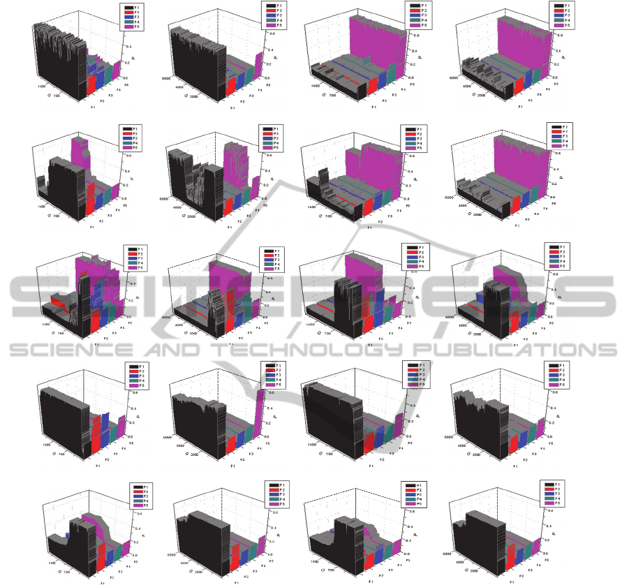
Figure 1: Dynamic change of distributions of
P
.
REFERENCES
Friedberg, R. M., (1958). A learning machine: Part I. IBM
Journal of Research and Development, 2, 2–13.
Box, G. E. P., (1957). Evolutionary operation: A method
for increasing industrial productivity. Applied
Statistics, 6, 81–101.
Holland, J. H., (1962). Outline for a logical theory of
adaptive systems. Journal of the Association for
Computing Machinery, 3, 297–314.
Fogel, L. J., (1962). Autonomous automata. Industrial
Research, 4, 14–19.
Storn, R. and Price, K., (1995). Differential evolution: a
simple and efficient adaptive scheme for global
optimization over continuous spaces. Technical Report
TR-95-012, International Computer Science Institute,
Berkeley.
Storn, R., (1996). Differential evolution design of an IIR-
filter. In Proceedings of IEEE International
Conference on Evolutionary Computation (pp. 268–
273).
Storn, R., (2005). Designing nonstandard filters with
differential evolution. IEEE Signal Processing
Magazine, 22, 103–106.
Lakshminarasimman, L. and Subramanian, S., (2008).
Applications of differential evolution in power system
optimization. Studies in Computational Intelligence,
143, 257-273.
F1, 10-D F1, 30-D F2, 10-D F2, 30-D
F3, 10-D F3, 30-D F4, 10-D F4, 30-D
F5, 10-D F5, 30-D F6, 10-D F6, 30-D
F7, 10-D F7, 30-D F8, 10-D F8, 30-D
F9, 10-D F9, 30-D F10, 10-D F10, 30-D
IJCCI2012-InternationalJointConferenceonComputationalIntelligence
142

Lobo, F. G. and Goldberg, D. E., (2001). The parameter-
less genetic algorithm in practice. Technical Report
2001022, University of Illinois at Urbana-Champaign,
Urbana, IL.
Harik, G. R. and Lobo, F. G. (1999). A parameter-less
genetic algorithm. In Banzhaf et al. (Eds.),
Proceedings of the 1999 genetic and evolutionary
computation conference (vol. 1, pp. 258–265.),
Morgan Kaufmann: Orlando.
Gämperle, R., Müller, S. D. and Koumoutsakos, P.,
(2002). A parameter study for differential evolution. In
Grmela, and Mastorakis (Eds.), Advances in
Intelligent Systems, Fuzzy Systems, Evolutionary
Computation (pp. 293–298). WSEAS Press: Interlaken.
Omran, M. G. H., Salman, A. and Engelbrecht, A. P.,
(2005). Self-adaptive differential evolution. In Lecture
Notes in Artificial Intelligence (pp. 192–199),
Springer-Verlag: Berlin.
Brest, J., Greiner, S., Boskovic, B., Mernik, M. and
Zumer, V., (2006). Self-adapting control parameters in
differential evolution: A comparative study on
numerical benchmark problems. IEEE Transactions
on Evolutionary Computation, 10, 646–657.
Teo, J., (2006). Exploring dynamic self-adaptive
populations in differential evolution. Soft Computing-
A Fusion of Foundations, Methodologies and
Applications, 10, 637–686.
Qin, A. K., Huang, V. L, and Suganthan, P. N., (2009).
Differential Evolution Algorithm With Strategy
Adaptation for Global Numerical Optimization. IEEE
Transactions on Evolutionary Computation, 13, 398 –
417.
Price, K., Storn, R., and Lampinen, J., (2005). Differential
Evolution—A Practical Approach to Global
Optimization. Springer-Verlag: New York.
Rogalsky, T., Derksen, R. W., and Kocabiyik, S., (1999).
Differential evolutionin aerodynamic optimization. In
Proceedings of the 46th Annual Conference of the
Canadian Aeronautics and Space Institute (pp. 29–36),
Montreal.
Zaharie, D., (2003). Control of population diversity and
adaptation in differential evolution algorithms. In
Matousek and Osmera (Eds.), Proceedings of 9th
International Conference on Soft Computing (pp. 41–
46), Brno.
ReplicatorDynamicInspiredDifferentialEvolutionAlgorithmforGlobalOptimization
143
