
A Simulation Study of Learning a Structure
Mike's Bike Commuting
Mamoru Kaneko
1
, Jeffrey J. Kline
2
, Eizo Akiyama
1
and Ryuichiro Ishikawa
1
1
IPPS, University of Tsukuba, Tsukuba, Japan
2
Economics, University of Queensland, Brisbane, Australia
Keywords:
Inductive Game Theory, Social Simulation, Learning, Short-term Memory, Long-term Memory, Preferences.
Abstract:
This paper undertakes a simulation study of a player’s learning about the structure of a game situation. In a
simple 1-person example called Mike’s Bike Commuting, we simulate the process in which Mike experiences
and accumulates memories about the structure of Mike’s town. It is the basic requirement that to keep an
experience as a long-term memory, Mike needs enough repetitions of that experience. By the choice of our
simple and casual example, we can discuss relevant time spans for learning. The limit case of Mike’s learning
as time tends to infinity is of little relevance to the problem of learning. We find that the concept of “marking”
introduced by Kaneko-Kline is important for obtaining sufficient structural knowledge in a reasonable time
span. Our study shows that Mike’s learning can change drastically with the concept. We also consider Mike’s
learning about his preferences from his experiences, where we meet various new conceptual problems.
1 INTRODUCTION
This paper undertakes a simulation study of a player’s
learning about details of a social situation. It is moti-
vated by the research in inductive game theory (IGT)
initiated by (Kaneko and Matsui, 1999) and (Kaneko
and Kline, 2008). Those papers concentrated on the
inductive derivation of a personal view from his ac-
cumulated memories, without touching on the precise
processes of experiencing and accumulating memo-
ries. These processes are of a truly finite and complex
nature. To consider such processes, we adopt a sim-
ulation method. As far as we target the learning by
a single human player, the length of time should be
within his life time. A simulation study enables us to
consider this problem.
Now, we look at the original motivation for IGT
by comparing it with two main stream approaches in
the recent game theory literature: the classical ex ante
decision approach and the evolutionary/learning ap-
proach. The contrasts between them will be used to
motivate our use of a simulation study.
The focus of the classical ex ante deci-
sion approach is on the relationship between be-
liefs/knowledge and decision making (cf., (Harsanyi,
1967/68) for the incomplete information game and
(Kaneko, 2002) for the epistemic logic approach to
decision making in a game). In this approach, the be-
liefs/knowledge is given a priori without specifying
their sources.
Contrary to this, the evolutionary/learning ap-
proach (cf., (Weibull, 1995) and (Fudenberg and
Levine, 1998)) targets experiential worlds more.
However, this approach does not ask the question
of the emergence of beliefs/knowledge. Instead,
their concern is typically the convergence of the
distribution of actions to some equilibrium. The
term “evolutionary/ learning” means that some effects
from past experiences remain in the distribution of
genes/actions. It is not about an individual’s con-
scious learning of the details of the game; typically it
is not specified who the learner is and what is learned.
When we work on an individual’s learning, we should
make these questions explicit.
If the learner is an ordinary person, the conver-
gence of behavior is not very relevant to his learn-
ing. Finiteness of life and learning must be crucial.
Here, relevant “finite” is “shallowly finite” rather than
the standard “finite” in mathematics. Consequently,
we conduct simulations over finite spans of time cor-
responding to the learning span of a single human
player. Our simulation indicates various specific com-
ponents affecting one’s finite learning, while they are
not relevant in the limiting behavior.
In this paper, we focus on the transformation from
raw experiences to accumulated memories. This part
208
Kaneko M., J. Kline J., Akiyama E. and Ishikawa R..
A Simulation Study of Learning a Structure - Mike’s Bike Commuting.
DOI: 10.5220/0004053602080217
In Proceedings of the 2nd International Conference on Simulation and Modeling Methodologies, Technologies and Applications (SIMULTECH-2012),
pages 208-217
ISBN: 978-989-8565-20-4
Copyright
c
2012 SCITEPRESS (Science and Technology Publications, Lda.)

was discussed as informal basic postulates in (Kaneko
and Kline, 2008). The social situation we take for our
simulation study is much simpler than the theoreti-
cal development of IGT in (Kaneko and Kline, 2008).
Nevertheless, the study of this paper highlights what
kinds of difficulties are involved in accumulation of
memories and how we should proceed with our re-
search in IGT.
Now, we discuss several points pertinent to our
simulation model.
(1) An Ordinary Person and an Every-day Situation
in a Social World. We target the learning of an ordi-
nary human person in a repeated every-day situation,
which we regard only as a small part of the entire so-
cial world for that person. We choose a simple and
casual example called “Mike’s Bike Commuting”. In
this example, the learner is Mike, and he learns the
various routes to his work. Using this example, the
time span and the number of reasonable repetitions
for the experiment become explicit.
(2): Ignorance of the Situation. At the beginning,
Mike has no prior beliefs/knowledge about the town.
His colleague gave a coarse map of possible alterna-
tive routes without precise details, and suggested one
specific route from his apartment to the office. Mike
can learn the details of these routes only if he expe-
riences them. We question how many routes Mike is
expected to learn after specific lengths of time.
(3) Regular Route and Occasional Deviations. Mike
usually follows the suggested route, which we call the
regular route. Occasionally, when the mood hits him,
he takes a different route. This is based on the ba-
sic assumption that his energy/time to explore other
routes is scarce. Commuting is only a small part of
his social world, and he cannot spend his energy/time
exclusively exploring those routes.
(4) Short-term and Long-term Memories. We distin-
guish two types of memories for Mike: short-term and
long-term. Short-term memories form a finite time
series consisting of past experiences, and they will be
kept only for some finite length of time, perhaps a few
days or weeks; after then they will vanish. However,
when an experience occurs with a certain frequency,
it becomes a long-term memory.Long-term memories
are lasting.
In our theory, the transition from a short-term to
a long-term memory requires some repetition of the
same experience within a given period of time. This
is based on the general idea that memory is reinforced
by repetition. Our formulation can be regarded as a
simplified version of Ebbinghous’ retention function
(Ebbinghous, 1964, 1885).
(5) Finiteness and Complexity. Our learning process
is formulated as a stochastic process. Unlike other
learning models, we are not interested in the conver-
gence or limiting argument. As stated above, the time
structure and span are finite and short. In our ex-
ample, we discuss how many times Mike has experi-
enced a particular route after a half year, one year, or
ten years. We will find many details, which are highly
complex even in this simple example. We analyze
those details and find the lasting features in Mike’s
mind.
(6) Marking Salient Choices as Important. Although
the situation is extremely simple, it is difficult for
Mike to fully learn the details of the entire town even
after several years. We consider the positive effect
on learning by “marking”, introduced in (Kaneko and
Kline, 2007). If Mike marks some “salient” choice
as “important”, and restricts his trial-deviations to the
marked choices, then we find that his learning is dras-
tically improved. Imperfections in a player’s memory
make marking important for learning. Without mark-
ing, experiences are infrequent and lapse with time.
Consequently, his view obtained from his long-term
experiences could be poor and small. By marking, he
focuses his attention on fewer choices, and success-
fully retains more as long-term memories.
Up to here, we study how many commutingsMike
needs in order to lean some routes. Precise objects
Mike possibly learn are not targeted here. There are
two directions of a departure from this study. One
possibility is to study Mike’s learning of internal com-
ponents of routes, and the other is about relationships
between routes. Of course, to study both in an in-
teractive way is possible. In this paper, however, we
consider a problem categorized to the latter. That is,
we consider Mike’s learning of his own preferences
from experiences and involved problems.
(7) Learning Preferences. Here, we face new concep-
tual problems. We should make a distinction between
having preferences and knowing them. We assume
that Mike has well-defined complete preferences, but
his knowledge is constrained to only some part by
his experiences. Learning one’s preferences differs
from keeping a piece of information. Since the feel-
ing of satisfaction is relative and likely to be more
transient than the perception of a piece of informa-
tion, we hypothesize that learning one’s preferences
needs comparisons of outcomes close in time. Con-
sequently, marking alternatives becomes even more
important for obtaining a better understanding of his
own preferences.
In our simulation study up to Section 4, we will
get some understanding of relevant “shallowly finite”
time spans for ordinary life learning. Our study on
learning preferences in Section 5 is more substantive
ASimulationStudyofLearningaStructure-Mike'sBikeCommuting
209
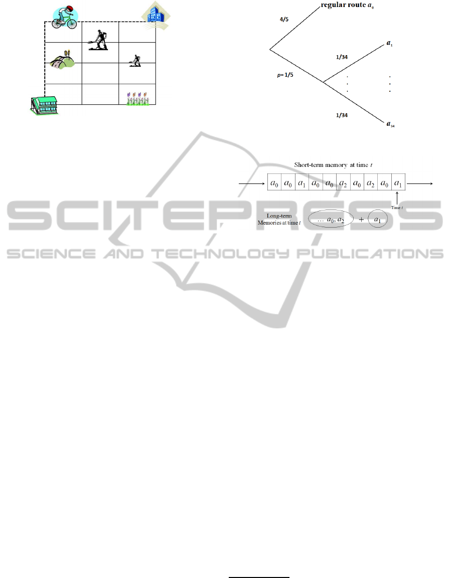
Figure 1: A map of the town.
than the studies up to Section 4. We will not go to the
direction to a study of learning of internal structures
of routes. This will be briefly discussed in Section 6.
2 MIKE'S BIKE COMMUTING
Mike moves to a new town and starts commuting to
his office everyday by a bike. At the beginning, his
colleague gives him a simple map depicted as Fig.1
and indicates one route shown by the dotted line.
Mike starts commuting every morning and evening,
five days a week, that is, 10 times a week. From
the beginning, he wants to know the details of those
routes, but the map is simple and coarse. He decides
to explore some alternative routes when the mood hits
him, but typically he is too busy or tired and resorts to
the regular route suggested by the colleague.
The town has a lattice structure: His apartment
and office are located at the south-west and north-east
corners. To have a route of the shortest distance from
his apartment to the office, he should choose “North”
or “East” at each lattice point; such a route is called a
direct route. There are 35 direct routes. He enumer-
ates these routes as a
0
,a
1
,...,a
34
, where a
0
denotes
the regular route.
In our simulation, we assume that Mike follows a
0
with probability 4/5 = 1− p and he makes a deviation
to some other route with p = 1/5. This probability p
is called the deviation probability. When he makes a
deviation, he chooses one route from the remaining 34
routes with the same probability 1/34. His behavior
each morning or evening can be depicted by the tree
in Fig.2. In sum, on average, he makes a deviation
twice a week to any of the other routes with equal
probability.
After taking route a
l
, he gets some impressions
and understanding of a
l
. In this paper we do not study
the details of a
l
that he learns; instead, we study con-
ditions for an experience to remain in his mind as a
long term memory.
As mentioned in Section 1, he has two types of
Figure 2: Decision tree in each trip of commuting.
Figure 3: Short-term and long-term memories.
memories: short-term and long-term. A short-term
memory is a time series of experiences of the past m
trips. An experience disappears after m trips of com-
muting. If the same experience, say a
l
, occurs at least
k times in m trips, experience a
l
becomes a long-term
memory. Long-term memories form a set of experi-
ences without time-structure or frequency.
1
In our simulation, we specify the parameters
(m,k) as (10,2), meaning that Mike’s short-term
memory has length 10, and if a specific experience
occurs at least two times in his short-term memory, it
becomes a long-term memory. This situation is de-
picted in Fig.2, where at time t − 1, the routes a
0
,a
2
are already long-term memories, and at time t, route
a
1
becomes a new long-term memory.
We consider another parameter T, denoting the to-
tal number of trips (time span). For example:
after 0.5 year, T = 2 × 5 (days) × 25 (weeks) = 250;
after 1 year, T = 2× 5 × 50 = 500;
after 10 years, T = 2× 5 × 500 = 5000.
Our simulation will be done by focussing on the half
year and 10 year time spans. In Mike’s Bike Commut-
ing, the number of available routes is 35, but later, this
will also be changed, and the number of routes will be
denoted as a parameter s. Listing all the parameters,
1
This lack of time structure and frequency is motivated
by bounded rationality of the player. Limitations on his
memory and computation abilities lead him to ignore some
aspects like the time structure and frequency of long term
memories.
SIMULTECH2012-2ndInternationalConferenceonSimulationandModelingMethodologies,Technologiesand
Applications
210

we have our simulation frame F:
F = [s, p;(m,k)]. (1)
We always assume that in the case of a deviation, a
route other than a
0
is chosen with equal probability
1/(s− 1).
The stochastic process is determined by the sim-
ulation frame F and a given T, which consists of T
component stochastic trees depicted in Fig.2. This
process is denoted by F[T] = [s, p;(m,k) : T]. Our
concern is the probability of some event of long-
term memories at time T. For example, what is the
probability of the event that a particular route a
l
is a
long-term memory at T? Or, what is the probability
that all routes are long-term memories? We calcu-
late those probabilities by simulation. In Section 3,
we give our simulation results for F = [s, p;(m,k)] =
[35,1/5;(10,2)] and T = 250,5000.
Before going to these results, we mention one
analytic result: For the stochastic process F[T] =
[35,1/5;(10,2) : T],
the probability that all routes become long-term
memories tends to 1 as T tends to infinity. (2)
This can be proved easily because the same experi-
ence occurs twice in a short-term memory at some
point of time almost surely if T is unbounded. This
result does not depend on the specification of param-
eters of F. Our interest, however, is in finite learning.
Our findings by simulation for the finite learning pe-
riods of T = 250 and T = 5000 differ significantly
from the above convergence result. This suggests that
focussing on convergence results does not inform us
about finite learning.
3 PRELIMINARY SIMULATIONS
AND THE METHOD OF
SIMULATIONS
We start in Section 3.1 by giving simulation results
for the case of s = 35. The results show that it would
be difficult for Mike to learn all the routes after a half
year. After ten years, he learns more routes, but we
cannot say much about which specific routes he learns
other than the regular one. In Section 3.2, we give a
brief explanation of our simulation method and the
meaning of “probability”.
3.1 Simulation Results for s = 35
Consider the stochastic process determined by F =
[s, p : (m,k)] = [35,1/5;(10,2)] for up to T = 250 (a
half year) and T = 5000 (10 years). Table 1 provides
the probabilities of the event that a specific route a
l
is a long-term memory at T = 250,5000, and also at
a large T : The row for a
0
shows that the probability
Table 1.
T 250 5000 28252 (> 56 years)
a
0
1 1 1
a
l
(l 6= 0) 0.069 0.765 0.99
of the regular route a
0
being a long-term memory is
already 1 at T = 250 (a half year). This “1” is still an
approximation result meaning it is very close to 1.
The row for a
l
(l 6= 0) is more interesting. The
probability that a specific a
l
is a long-term memory at
T = 250 and 5000 is 0.069 and 0.765, respectively.
Our main concern is to evaluate these probabilities
from the viewpoint of Mike’s learning.
Some reader may have expected that the proba-
bility for T = 250 would be much smaller than 0.069,
because in each trip, the probability of route a
l
(l 6= 0)
being chosen is only 1/5×1/34 = 1/170 = 0.00588.
However, it is enough for a
l
to occur in a consec-
utive sequence of length 10 (short-term memory) at
some t ≤ 250, and there are 240 such consecutive se-
quences. Hence, the probability turns out not to be
negligible. The accuracy of this calculation will be
discussed in Section 3.2.
The rightmost column is prepared for a purpose of
reference. The number of trips 28252 (> 56 years) is
obtained from asking the time span needed to obtain
the probability 0.99 of a
l
(l 6= 0) being a long-term
memory. The length of 56 years would typically ex-
ceed an individual career, and thus we regard the lim-
iting convergence result (2) as only a reference (the
model without decay of long-term memories may be
inappropriate for 56 years).
We next look more closely at the distribution of
routes he learns for each of those time spans.
For T = 250, we give Table 2, which describes
the probability of exactly r routes (the regular route
and r − 1 alternative routes) being long-term memo-
ries in 35 routes: After r = 5 routes, the probability
is diminishing quickly, so we exclude those numbers
from the table. According to our results, Mike typi-
cally learns a few routes (the average is about 3.33)
after half a year. For r = 3, one route must be regu-
lar, but the other two are arbitrary. This means that
although Mike learns about 2 alternative routes, it is
hard to predict with much accuracy which pair would
Table 2.
r 1 2 3 4 5 ···
0.089 0.223 0.272 0.213 0.121 · ··
ASimulationStudyofLearningaStructure-Mike'sBikeCommuting
211

be learned.
At T = 5000, i.e., ten year later, Mike’s learning
is described by Table 3. Again, we show only the
Table 3.
r ·· · 25 26 27 28 29 ···
··· 0.109 0.159 0.153 0.153 0.124 ···
values of r having high probabilities. The average of
the number of routes as long-term memories is about
27. Because most of the distribution lies between 25
and 29 routes, we find that there are many more cases
to consider than after half a year. For example, con-
sider 0.109 for r = 25, which is the probability that
exactly 25 routes are learned. This probability can be
obtained from the probability 0.765 in Table 1 by the
equation:
34
24
× (0.765)
24
× (1− 0.765)
10
+ 0.109.
Looking at this equation, we obtain the probability
that a specific set of 25 routes are long-term memo-
ries is only 0.109/
34
24
= 8.31× 10
−10
. In sum, Mike
learns about 27 alternativeroutes after 10 years. How-
ever, the number of combinationsof 24 routes from 34
is enormous at about 1.3× 10
8
and much larger than
the
34
2
= 561 cases we need to consider after only
half a year.
Finally, we report the average time for Mike to
learn all the 35 routes as long-term memories, which
is 28.4 years (14,224.3 trips). If he is very lucky, he
will learn all routes in a short length of time, say, 10
years, which is an unlikely event of probability 9 ×
10
−5
. The probability of having learned all routes in
35 years is much higher at 0.806.
After all, the above calculations indicate that
“finiteness” involved in our ordinary life is far from
“large finiteness” appearing in the convergence argu-
ment in mathematics. In this sense, we are facing
shallowly finite problems, which was emphasized in
Section 1. In Sections 4 and 5, we will discuss related
problems to this issue from different perspectives.
3.2 Simulation Method
We now explain the concept of “probability” we are
using, and discuss the accuracy of this concept. First
we mention why this is not calculated in an ana-
lytic manner. The analytic computation is feasible
up to about T = 30, but beyond T = 40, it is practi-
cally impossible in the sense that for T = 50, it takes
more than 100 years to calculate with current (year
2007) computers using our analytical method. This
Figure 4: A simulation up to T = 250.
is caused by the limited length of short-term mem-
ory and multiple occurrences needed for a long-term
memory.
We take the relative frequency of a given event
overmany simulation runs instead of computing prob-
abilities analytically. We use the Monte Carlo method
to simulate the stochastic process up to a specific T
for the simulation frame F = [s, p : (m,k)] = [35,1/5 :
(10,2)]. The frame has only two random mechanisms
depicted in Fig.2, but they are reduced into one ran-
dom mechanism. This mechanism is simulated by
a random number generator. Then, we simulate the
stochastic process determined by F up to T = 250 or
T = 5000 or some other time span. A simulation is
depicted in Fig.4. One simulation run gives a set of
long-term memories: In Fig.4, routes a
0
,a
2
,a
3
,a
5
are
long-term memories at some time before T = 250.
We run this simulation 100,000 times. The “prob-
ability” of a
l
is calculated as the relative frequency:
#{simulation runs with a
l
as a long-term memory}
100, 000
(3)
In the case of T = 250, this frequency is about 0.069
for l 6= 0, and it is already 1 for l = 0 in our simulation.
We compare some results from simulation with
the results obtained by the analytical method. For
T = 20 and s = 35, the probability of a
l
being a long-
term memory can be calculated in an analytic man-
ner using a computer. The result coincides with the
frequency obtained using simulation to an accuracy
of 10
−4
. In sum, we calculate the “probability” of an
event as the relative frequency over numerous simu-
lation runs.
4 LEARNING WITH MARKING:
SIMULATION FOR S = 5
We now show how “marking”, introduced in (Kaneko
and Kline, 2007), can improve Mike’s learning. By
concentrating his efforts on a few “marked” routes,
he is able to learn and retain more experiences. This
is because the likelihood of repeating an experience
SIMULTECH2012-2ndInternationalConferenceonSimulationandModelingMethodologies,Technologiesand
Applications
212

rises by reducing the number of alternative routes. In
Section 4.1, we consider the case where Mike marks
only four alternative routes in addition to the regular
one. We see a dramatic increase in his learning of al-
ternative routes. In Section 4.2, we show how a more
planned approach can improve the effect of “mark-
ing” on his learning.
4.1 Marking Five Salient Routes and
Simulation Results
Figure 5: Five marked routes.
Suppose that Mike decides to mark some routes
from his map for his exploration. He uses two criteria:
(i) he chooses routes having a scenic hill or flowers;
(ii) he avoids construction sites.
Then, he marks only four alternativeroutes, which are
depicted in Fig.5. Adding the regular route a
0
, we
denote the five marked routes by a
0
,a
1
,a
2
,a
3
,a
4
.
The above situation is described by changing the
simulation frame to F = [s, p : (m,k)] = [5,1/5 :
(10,2)] for T = 250 or 5000. The probability of a
l
(l 6= 0) being a long-term memory is calculated by
our simulation method and is given in Table 4: Table
Table 4.
T 250 5000
s = 5 0.970 1.00
s = 35 0.069 0.765
Table 5.
T 425 28253
s = 5 0.990 1.000
s = 35 0.114 0.990
5 lists the length of time needed to obtain the prob-
ability 0.99 that an alternative route a
l
(l 6= 0) is a
long-term memory. With marking he needs only 425
trips (10.2 months), as opposed to the 28,253 trips
(more than 56 years) without marking.
We also have calculated, and presented in Table 6,
the probability that exactly r (= 1,2,3,4, 5) routes are
long-term memories at T = 250. The average number
of routes learned is 4.9. Table 7 states that the average
time for Mike to learn all 35 routes is about 100 times
the average time to learn 5 routes by marking. This
suggests that Mike might be able to use marking in
a more sophisticated manner to learn all 35 routes in
a shorter period of time than the 28.4 years required
without marking. We will look more closely at this
idea in Section 4.2.
Table 6.
r 1 2 3 4 5
8.00× 10
−7
1.04× 10
−4
5.05× 10
−3
0.109 0.886
Table 7.
s = 5 s = 35
the average number of
trips to learn all
151.8
3.6 months
14,224.3
28.4 years
4.2 Learning by Marking and Filtering
Suppose that Mike has learned all four marked alter-
native routes in addition to the regular route after a
half year. He may then want to explore some other
routes. He might plan to explore the other 30 routes
by dividing them into 6 bundles of 5 routes, trying
to learn each bundle one by one. We suppose that
he explores one bundle for a half year, and he moves
to the next bundle storing any long-term memories in
the process. Thus, Mike has discovered a method of
filtering to improve his learning.
According to the result of Section 4.1, Mike most
likely learns all five routes within a half year. By his
filtering he reduces the expected time to learn all 35
routes from 28.4 years to only 250 × 7 = 1750 (3.5
years).
The probability of that he finishes his entire ex-
ploration in 3.5 years is (0.886)
7
+ 0.427, and with
the remaining probability 0.573, at least one route is
not learned after 3.5 years. If some routes still remain
unlearned, then we assume that he rebundles the re-
maining routes into bundles of 5. However, we expect
a rather small number of unlearned routes to remain;
the event of 3 remaining is rare event occurring with
only probability 0.03. With high probability, Mike’s
learning finishes within 4 years.
If we treat the above filtering method alone, for-
getting the original constraint such as the energy-
scarcity mentioned in Section 1, the extreme case
would be that he chooses and fixes one route for two
trips and goes to another route. In this way, he could
learn all routes with certainty in precisely 35 days.
However, this type of short-sighted optimal program-
ming goes against our original intention of explo-
ration being rather rare and unplanned. Commuting
is one of many everyday activities for Mike, and he
ASimulationStudyofLearningaStructure-Mike'sBikeCommuting
213

cannot spend his energy/time exclusively on planning
and undertaking this activities. Though our example
is very simplified, we should not forget that many un-
written constraints lie behind it.
5 LEARNING PREFERENCES
Here, we consider Mike’s learning of his own pref-
erences. Mike finds his own preferences based on
comparisons between experienced routes. First, we
specify the bases for our analysis, and then we formu-
late the process in which Mike learns his own pref-
erences. We simulate this learning process in Sec-
tion 5.1, and show that learning of his preferences
is typically much slower than learning routes. Con-
sequently, notions like “marking” become even more
important. In Section 5.2, we consider the change of
the process when he adopts a more satisfying route
based on his past experiences.
5.1 Preferences
Since Mike has no idea of details along each route
at the beginning, one might wonder if he has well-
defined preferences over the routes or what form they
would take. By recalling the original meaning of
“preferences”, however, we can connect them with
experiences. Since an experience of each route gives
some level of satisfaction, comparisons between sat-
isfaction levels can be regarded as his preferences.
Here, preferences are assumed to be inherent, but they
are only revealed to Mike himself when he experi-
ences and compares different outcomes. In this way,
Mike may come to knowsome of his own preferences.
We assume that Mike’s inherent preference rela-
tion over the routes is complete and transitive. A
preference between two routes is experienced only
by comparing the two satisfaction levels from those
routes.
2
A feeling of satisfaction typically emerges in
the mind (brain) without tangible pieces of informa-
tion. Such a feeling may often be transient and only
remain after being expressed by some language such
as “this wine is better than yesterday’s”. We assume,
firstly, that satisfaction is of a transient nature, and
secondly, that the satisfaction from one route can be
compared with that of another only if these have hap-
pened closely in time.
2
This should be distinguished from “revealed prefer-
ences” (cf. (Malinvaud, 1972)) where a preference is de-
fined by a (revealed) choice from hypothetically given two
alternatives. This hypothetical choice is highly problematic
from the experiential point of view.
We formulate a preference comparison between
two routes as an experience. This experience has
a quite different nature from a sole experience of a
route. The former needs the comparison of two ex-
perienced satisfaction levels. To distinguish between
these different types of experiences, we call a sole ex-
perience of a route a first-order experience, while a
pairwise comparison of two routes is a second-order
experience. Our present target is second-order expe-
riences.
Consider Mike’s learning of such second-order
experiences in the simulation frame F = [s, p :
(m,s)] = [5,1/5 : (10,2)] with T = 250 or 5000. A
short-term memory is now treated as a sequence of
length 10. Consecutive routes can be compared to
form preferences over pairs. For example, in Ta-
ble 8, the short-term memory is the sequence of 10
pairs ha
1
,a
0
i,ha
0
,a
0
i,...,ha
3,
a
0
i. We treat them as
unordered pairs, e.g., the pairs ha
1
,a
0
i and ha
0
,a
1
i in
t − 9 and t − 5 are treated as the same. These second-
order experiences may become long-term memories.
For a second-order experience to become a long-
term memory, however, it must occur at least twice
in a short-term memory. In Table 8, ha
0
,a
1
i occurred
twice, and hence it becomes a long-term memory. We
require these consecutive unordered pairs be disjoint;
for example, (a
0
,a
3
) and (a
3
,a
0
) occurred twice hav-
ing the intersection a
3
, so these occurrences are not
counted as two.
The computation result is given in Table 9 with
l, l
′
= 1,2,3,4 and l 6= l
′
. In the column of a
0
vs.
a
l
, the probability of the preference between a
0
and
a
l
being a long-term memory is given as 0.981 for
T = 250. After only about 2 years, the probability is
already 1
3
.
We find in the right column of Table 9 that Mike’s
learning is very slow. After a half year, Mike hardly
learns any of his preferences between alternative
routes. An experience of comparison between a
l
vs.
a
l
′
happens with such a small probability, because
both deviations a
l
and a
l
′
from the regular route a
0
are required consecutivelyand also twice disjointedly.
This means that his learned preferences are very in-
complete even after quite some time.
For example, suppose that Mike’s original prefer-
ence relation is the strict order, a
3
,a
4
,a
0
,a
1
,a
2
with
a
3
at the top, which is depicted as the left diagram
3
One might wonder why the value of 0.981 for a com-
parison between a
0
and a
l
is higher 0.970 for just learning
a route a
l
in Table 4. This can be explained by the counting
of pairs at the boundary. For example, the comparison be-
tween a
0
and a
1
appearing in Table 8 becomes a long-term
memory from the short-term memory at timet. However, in
our previous treatment of memory of routes, a
1
would not
be a long-term memory.
SIMULTECH2012-2ndInternationalConferenceonSimulationandModelingMethodologies,Technologiesand
Applications
214

Table 8.
a
1
a
1
a
0
a
0
a
0
a
0
a
0
a
0
a
0
a
0
a
1
a
1
a
2
a
2
a
0
a
0
a
0
a
0
a
3
a
3
a
0
→ t − 9 t − 8 t − 7 t − 6 t −5 t − 4 t − 3 t − 2 t − 1 t →
Table 9.
trips
Prob. of
comparison
a
0
vs. a
l
Prob. of
comparison
a
l
vs. a
l
′
250 (a half year) 0.981 0.053
5000 (10 years) 1.000 0.671
10000 (20 years) 1.000 0.892
Table 10.
a
3
a
4
a
0
(reg.)
a
1
a
2
=⇒
a
3
a
4
(reg.)
տ ր
a
0
ր տ
a
1
a
2
=⇒
a
3
(reg.)
↑
a
4
↑
a
0
ր տ
a
1
a
2
of Table 10. After half a year, he likely learns his
preferences between a
0
(regular) and each alternative
a
l
,l = 1,2,3, 4, which is illustrated in the middle dia-
gram of Table 10. It is unlikely that he learns which
of a
3
or a
4
(or, a
1
or a
2
) is better. Even if he be-
lieves transitivity in his preferences, he would only
infer from his learned preferences that both a
3
and a
4
are better than a
1
and a
2
.
Ten years later, Mike’s knowledge will be much
improved. By this time, with probability 1, he will
have learned his preferences between a
0
and each
alternative a
l
,l = 1,2,3, 4. He will also likely have
learned his preferences between some of the alterna-
tives. Table 11 lists the probabilities that exactly r
of his preferences are learned. Recall that there are
5
2
= 10 comparisons. Even after 10 years, Mike
is still learning his own preferences over alternative
routes.
After 20 years, however, he learns much more
about his preferences, which is described in Table 12.
As it happens, by the time Mike is able to get to taste
the rough with the smooth, he is already old.
5.2 Maximizing Preferences
The results of the previous subsection tell us that it is
difficult for Mike to learn his complete preferences.
However, completeness should not be his concern.
For him, it would be important to find a better route
than the regular one, and to change his regular behav-
ior to the best route he knows. This idea is formulated
as follows:
(1): he continues to learn his preferences until he can
compare each marked alternative to the regular one;
(2): if he finds a better route a
l
than a
0
in those
comparisons, then he chooses a
l
(arbitrarily, if there
are multiple) as the new regular route;
(3): he stores a
0
and the alternative routes less pre-
ferred than a
0
;
(4): he makes an exploration of his preferences over
the remaining marked alternatives with the new regu-
lar route a
l
;
(5): he repeats the process determined similarly by
(1) − (4) until he does not find a better route than the
regular one.
The final result of this process gives a highest pref-
erence. Our concern is the length of time for this
process to finish, and his knowledge about his pref-
erences upon finishing.
Suppose that Mike’s original (hidden) preferences
are described by the left column of Table 10; he has
a strict preference ordering a
3
≻ a
4
≻ a
0
≻ a
1
≻ a
2
,
where a
0
is the regular route. After some time, he
learns his preferences described in the middle dia-
gram. In this case, it is very likely that only his pref-
erences between a
0
vs. a
l
(l 6= 0) are learned. The
arrow → indicates the learned preferences.
Here, let us see the average time to finish his learn-
ing for preference maximization, under the assump-
tion that as soon as he finishes his learning of the
preferences between the regular route and alternative
ones, he moves to learning the unlearned part. The
transition from the left column to the middle one in
Table 10 needs the average time 136.2 (3.3 months).
When he reaches the middle diagram, he stores the
preferences over a
0
,a
1
and a
2
.
In the middle diagram of Table 10, he starts com-
paring between a
3
and a
4
. Here, a
4
is taken as the new
regular route. Once he obtains the preference between
a
3
and a
4
, he goes to the right diagram and he plays
the most preferred route a
3
. The average time for this
second transition is 11.0 trips (1.1 week). Hence, the
transition from the left diagram of knowing no prefer-
ences, to the rightmost diagram takes the average time
of 136.2 + 11.0= 147.2 trips (3.5 months).
We have 5! = 120 possible preference orderings
over a
0
,a
1
,a
2
,a
3
,a
4
and a
5
. We classify them into
5 classes by the position of a
0
. Here we consider
only the other two cases: a
0
is the top or the bottom.
When a
0
is the top, only one round of comparing a
0
to other a
l
is enough to learn that a
0
is his most pre-
ferred route. This takes the average time 136.2 (3.3
months), which is the same as the time for the tran-
ASimulationStudyofLearningaStructure-Mike'sBikeCommuting
215

Table 11: 10 years.
r 4 5 6 7 8 9 10
1.07× 10
−3
0.0155 0.079 0.215 0.329 0.269 0.0913
Table 12: 20 years.
r 4 5 6 7 8 9 10
1.59× 10
−15
7.86× 10
−5
0.0016 0.0179 0.111 0.366 0.504
sition to the middle of Table 10. In the case with the
top a
0
, however, Mike learns no other preferences.
Consider the case where a
0
is the bottom. There
are several cases depending upon his choice of new
regular routes. But now there are four possibilities
for the choice of the next regular route. Depending
upon this choice, he may finish quickly or needs more
rounds. The more quickly he finishes, the more in-
complete are his preferences. Alternatively, the slow-
est case for finding the top needs 4 transitions. Table
13 depicts the slowest case: The total average time is
136.2+78.0+ 36.4+11.0= 261.6 (6.3 months); the
bold letter means the regular route. By this process he
finds his complete preferences, still, with the help of
transitivity.
In Sum, if Mike learns the top quickly, he learns
virtually nothing about his preferences between the
other alternatives. On the other hand, if he finds the
top slowly, he would have a much richer knowledge
of his own preferences.
Table 13: Transitions with learning preferences.
a
1
a
2
a
3
a
4
a
0
=⇒
a
1
a
2
a
3
a
4
տ↑ ↑ր
a
0
=⇒
a
1
a
2
a
3
տ տ ր
a
4
↑
a
0
=⇒
a
1
a
2
տ ↑
a
3
↑
a
4
↑
a
0
=⇒
a
1
↑
a
2
↑
a
3
↑
a
4
↑
a
0
6 CONCLUDING DISCUSSIONS
“Mike’s Bike Commuting” is a small everyday situa-
tion that provides insights to our everyday behavior.
We explicitly formulated and computed what learn-
ing is possible and relevant to a person within his life
span. Also, our target situation is partial relative a
player’s entire social world. This explains the regular
behavior as a consequence of time/energy saving and
also infrequent deviations as an exploration behavior.
Let us consider the implications of our study to
game theory. Our original motivation was, from
the viewpoint of IGT, to study the origin/emergence
of beliefs/knowledge of the structure of the game.
Long-term memories are the source for such be-
liefs/knowledge. Our results have the implication that
it would be difficult for a player to learn the full struc-
ture of a game, unless it is very simple. Even with
marking, the learning will typically be limited. This
suggests that different players will likely develop dif-
ferent views. One direction of theoretical research is
given in (Kaneko and Kline, 2007).
It is a negative but important implication that the
focus on limiting cases is no longer appropriate. This
leads us to deviate entirely from the learning litera-
ture in game theory (cf., (Weibull, 1995) and (Fuden-
berg and Levine, 1998)): This literature has typically
treated convergences; even though it starts from finite
worlds, it does not touch “shallowly finite” problems.
It is a positive implication that our research is more
related to everyday memory in the psychology liter-
ature (cf., (Linton, 1982) and (Cohen, 1989)). Yet,
there is a large distance between our study of IGT to-
gether with the present simulation and experimental
psychology. To build a bridge between those fields,
we need still to develop our theory as well as simula-
tion study.
There are various extensions to be considered for
future possible studies. Here, we discuss only two
such extensions.
Aspect 1: Long-term Memories and Decaying: It is
assumed that once an experience becomes a long-term
memory, it will last forever. However, it would be
more natural to assume that even long-term memo-
ries are subject to decay unless they are experienced
once in a while. In particular, when the regular behav-
ior changes as in Section 5.2, decay or forgetfulness
about past regular behavior might become important.
This remark is relevant to the problem of Section 4.2.
SIMULTECH2012-2ndInternationalConferenceonSimulationandModelingMethodologies,Technologiesand
Applications
216

1
0
t
Retention
probability
1
2
3
Figure 6: Ebbinghous’s retention function.
This problem is related to Ebbinghous’ (Ebbing-
hous, 1964, 1885) retention function which was used
to describe experimental results of memory of a list of
nonsense syllables. No distinction is made between a
short-term memory and a long-term memory. The re-
tention function is typically considered as taking the
shape of any curved line depicted in Figure 6, where
the height denotes the probability of retaining a mem-
ory and it is diminishing with time
4
.
This direction may become more fruitful with
an experimental study such as in (Takeuchi, Funaki,
Kaneko, and Kline, 2011).
Aspect 2: Two or More Learners. We have concen-
trated our focus on the example of Mike’s Bike Com-
muting. We are interested in learning in game situa-
tions with two or more learners (players)
5
. This has
other new features like the relevant learning time. For
example, one may learn over his life time, but only
interact with another player for a shorter time span.
Also, how does his learning affect the other’s learn-
ing? We might start with the “small and partial views”
setting of (Kaneko and Kline, 2007), but expect that
communication and role switching will likely be im-
portant.
These are straightforward extensions but may ex-
pect a lot of implications to our study. We can even in-
4
His experiments are interpreted as implying that the
retention function may be expressed as an exponential
function. By careful evaluations of Ebbinghous’ data,
Anderson-Schooler (Anderson and Schooler, 1991) reached
the conclusion that the retention function can be better ap-
proximated as a power function, i.e., the probability of re-
taining a memory after time t is expressed as P = At
−b
.
5
(Hanaki, Ishikawa, Akiyama, 2009) studied the con-
vergence of behaviors in a 2-person game, where each
player’s learning of payoffs is formulated in the way of the
present paper but his behavior is formulated as a mechanical
statistical process following the learning literature. Then,
they studied behavior of outcomes in life spans of middle
range. Their approach did not take purely the viewpoint of
IGT in that a player consciously makes a behavior revision
once he has a better understanding of a game situation. Nev-
ertheless, it would give some hint to our further research on
IGT.
troduce more probabilistic factors related to decaying
of long-term as well as short-term memories. How-
ever, more essential extensions are related to the con-
sideration of internal structures of routes and induc-
tive derivations of individual views from experiences.
Simulation studies of those aspects provide a lot of
new directions for research and implications for IGT
as well as the extant game theory.
REFERENCES
Anderson J. R. and L. J. Schooler (1991), Reflections of
the environment in memory, American Psychological
Society 2, 396-408.
Cohen, G., M., (1989), Memory in the Real World,
Lawrence Erlbaum Associates Ltd. Toronto.
Ebbinghous, H., (1964, 1885), Memory: A contribution to
experimental psychology, Mieola, NY: Dover Publi-
cations.
Fudenberg, D., and D.K. Levine, (1998), The Theory of
Learning in Games, MIT Press, Cambridge.
Hanaki, N., R. Ishikawa, E. Akiyama, (2009), Learning
Games, Journal Economic Dynamics & Control 33,
1739-1756.
Harsanyi, J. C., (1967/68), Games with Incomplete Infor-
mation Played by ‘Bayesian’ Players, Parts I,II, and
III, Management Sciences 14, 159-182, 320-334, and
486-502.
Linton, M., (1982), Transformations of memory in every-
day life. In U, Neisser ed. Memory Observed: Rem-
bering in natural contexts. Freeman, San Francisco.
Kaneko, M., (2002), Epistemic Logics and their Game The-
oretical Applications: Introduction. Economic Theory
19, 7-62.
Kaneko, M., and J. J. Kline, (2007), Small and Partial
Views derived from Limited Experiences, University
of Tsukuba, SSM.DP.1166, University of Tsukuba.
Kaneko, M., and J. J. Kline, (2008), Inductive Game The-
ory: A Basic Scenario, Journal of Mathematical Eco-
nomics 44, 1332-1363.
Kaneko, M., and J. J. Kline, (2009), Partial Memories,
Inductively Derived Views, and their Interactions
with Behavior, to appear in Economic Theory, DOI:
10.1007/s00199-010-0519-0
Kaneko, M., and A. Matsui, (1999), Inductive Game The-
ory: Discrimination and Prejudices, Journal of Public
Economic Theory 1, 101-137. Errata: JPET 3, 347.
Malinvaud, E., (1972), Lectures on Microeconomic Theory,
North-Hollond. Amsterdam.
Takeuchi, A., Y. Funaki, M. Kaneko, and J. J. Kline,
(2011), An Experimental Study of Behavior and Cog-
nition from the Perspective of Inductive Game Theory,
SSM.DP.No.1267, University of Tsukuba.
Tulving, E., (1983), Elements of Episodic Memory, Oxford
University Press, London.
Weibull, J. W., (1995), Evolutionary Game Theory, MIT
Press. London.
ASimulationStudyofLearningaStructure-Mike'sBikeCommuting
217
