Observations of Discrete Event Models

Gauthier Quesnel

, Ronan Tr

epos

and

Eric Ramat

INRA, UR875 Biom

etrie et Intelligence Artiﬁcielle, F-31326 Castanet-Tolosan, France

ULCO, LISIC, 50 Rue Ferdinand Buisson BP 719, 62228 Calais Cedex, France

Keywords:

Simulation, Discrete Event Systems, DEVS Formalism, Observation, Methodology.

Abstract:

The observation of a simulation is an important task of the modeling and simulation activity. However, this

task is rarely explained in the underlying formalism or simulator. Observation consists to capture the state

of the model during the simulation. Observation helps understand the behavior of the studied model and

allows improving, analyzing or debugging it. In this paper, we focus on appending an observation mechanism

in the Parallel Discrete Event System Speciﬁcation (PDEVS) formalism with guarantee of the reproducible

simulation with or without observation mechanism. This extension to PDEVS allows us to observe models at

the end of the simulation or according to a time step. Thus, we deﬁne a formal speciﬁcation of this extension

and its abstract simulators algorithms. Finally, we present an implementation in the DEVS framework VLE.

1 INTRODUCTION

In the Modeling and Simulation (M&S) activity, ob-

servation of the behavior of models is an important

aspect. An observation captures the state or the evo-

lution of the state during or at the end of the simula-

tion. It allows the modeler to test, prove, validate, or

generate data from simulations by connecting simula-

tion software application to output streams like ﬁles,

databases, unit test or visualization software. Obser-

vations contribute to the modelers representation of

its studied system.

In environmental and agronomic modeling do-

main, we need to couple heterogeneous models.

These models can be continuous or discrete. In addi-

tion, these models co-exist in different temporal and

spatial scales. Thus, to solve this problem, we use

the Discrete Event Speciﬁcation System (DEVS) for-

malism (Zeigler et al., 2000). DEVS can be seen

as a common denominator for multi-formalism hy-

brid systems modeling (Vangheluwe, 2000). DEVS

takes place in the M&S theory deﬁned by B. P. Zei-

gler. M&S theory tends to be as general as possible.

It addresses major issues of computer sciences from

artiﬁcial intelligence to model design and distributed

simulations. M&S theory aims to develop a common

framework, formal and operational, for the speciﬁca-

tion of dynamical systems.

Modeling the observation process is dependent on

the underlying formalism. However, for many forma-

lisms, the observation does not exist and the outputs

of models are used directly. For example, the numeri-

cal integration method Euler used for solving ordinary

differential equations does not allow catching variable

between two time-steps. The observation process is

generally not explicit nor speciﬁed in the formalism.

Specify the observation process is generally not use-

ful. However, it becomes necessary when we want

to observe multi-models with the same observation

mechanism.

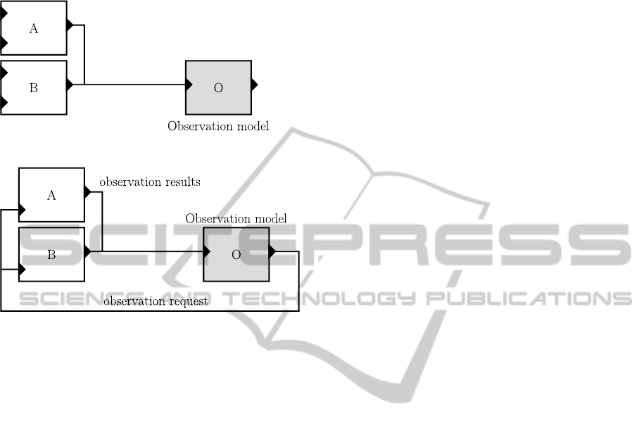
However, the DEVS formalism does not propose

observation of simulation models. Several solutions

exist without changing the behavior of DEVS. For

example, in the ﬁrst picture of the ﬁgure 1, outputs

of the models A and B are connected to an obser-

vation model O. O has a reactive behavior. Pow-

erDEVS (Bergero and Kofman, 2010) chooses this

solution. It is simple and has great ﬂexibility. How-

ever, it can be very expensive. Indeed, in the case

of experimental frames (to calibrate or estimate pa-

rameters or to optimize parameters on criteria), only

the ﬁnal values of the observations are necessary. All

the values received are useless. The interpretation of

these values can be costly. In the second picture of

the ﬁgure 1, an observation model O generates events

to observed models A and B. These models send

their outputs to the observation model. This solution

is computationally less expensive, but requires mix-

ing observation and normal behavior of the model.

This mechanism can induce a difﬁculty in reproduc-

Quesnel G., Trépos R. and Ramat É..

Observations of Discrete Event Models.

DOI: 10.5220/0004054300320041

In Proceedings of the 2nd International Conference on Simulation and Modeling Methodologies, Technologies and Applications (SIMULTECH-2012),

pages 32-41

ISBN: 978-989-8565-20-4

 2012 SCITEPRESS (Science and Technology Publications, Lda.)

ing simulations and can increase the complexity of

model.

Figure 1: Classical reactive and proactive observation

mechanism in DEVS.

We chose in this work to modify the DEVS for-

malism by adding an extension. This addition does

not change the behavior of DEVS. It adds a layer of

observation to DEVS. The DEVS trajectories of the

simulations are the same with or without this exten-

sion. However, some alternative exist to add an ob-

servation mechanism. Thus, rather than developing

the observation process in the formalism, researchers

developed this process in the software part of their

simulators. It is the choice made by JAMES 2 (Him-

melspach and Uhrmacher, 2009) and OSA (Ribault

et al., 2010). JAMES 2 uses the design pattern ob-

servation; OSA uses AOP (Aspect-oriented program-

ming. The design pattern observation links for each

model a list of observation component. This list has

a function called notify. The model calls this func-

tion when it wants to send observation value. The

observation component has a reactive behavior. This

type of behavior can increase the calculation to per-

form the treatment of observation values from multi-

models (e.g. Models that use formalism with different

time advance function). Of course, through a combi-

nation of the visitor and observer design patterns, we

can make active the behavior of the observation com-

ponent.

In this paper, we propose to extend the PDEVS

formalism with an observation mechanism. This ex-

tension to DEVS provides a generic way to observe

heterogeneous models and it guarantees the same sim-

ulations when this mechanism is activated and when

it is not.

This paper is divided into three parts. In the ﬁrst

part, we explain the PDEVS formalism. This formal-

ism is the context of our work. Then, we develop our

contribution in two parts. (1) We develop the for-

mal speciﬁcation of the observation extension. This

speciﬁcation guarantees to conserve the behavior of

PDEVS. (2) We present the abstract simulators of the

observation extension. Developers of PDEVS simula-

tors software can use these abstract simulators to in-

troduce the extension observation in their simulators.

The last sections show an implementation of this ex-

tension in the software VLE and an example of use.

Finally, we conclude this paper with conclusion and

perspectives.

2 METHOD

DEVS (Zeigler et al., 2000) is a well-known and ac-

cepted formalism for the speciﬁcation of complex dis-

crete or continuous systems abstracted as a network of

concurrent, timed and interacting models. DEVS pro-

vides a hierarchical and modular approach to model-

ing and simulation. The formalism supports two types

of models: atomic and coupled models. Atomic mod-

els interact thought a well-deﬁned set of input and

output values enabling a software component based

orientation to model representation. Atomic models

can be combined to form coupled models, providing

the constructs to the representation of complex mod-

els.

2.1 PDEVS Formalism

PDEVS (Chow and Zeigler, 1994) extends the Clas-

sic DEVS essentially by allowing bags of inputs to

the external transition function. Bags can collect in-

puts that are built at the same date, and process their

effects in future bags. This formalism offers a solu-

tion to manage simultaneous events that could not be

easily managed with Classic DEVS. For a detailed de-

scription, we encourage the reader to read the section

3.4.2 in chapter 3 and the section 11.4 in chapter 11

of Zeigler’s book (Zeigler et al., 2000).

PDEVS deﬁnes an atomic model as a set of input

and output ports and a set of state transition functions:

M =

X,Y,S, δ

int

,δ

ext

,δ

con

,λ, ta

With:

ObservationsofDiscreteEventModels

X is the set of input values

Y is the set of output values

S is the set of sequential states

ta : S → R

is the time advance function

int

: S → S is the internal transition function

ext

: Q × X

→ S is the external transition

function

Q = {(s, e)|s ∈ S,0 ≤ e ≤ ta(s)}

Q is the set of total states,

e is the time elapsed since last transition

is a set of bags over elements in X

con

: S × X

→ S is the conﬂuent transition

function, subject to δ

con

(s,

0) = δ

int

(s)

λ : S → Y is the output function

If no external event occurs, the system will stay

in state s for ta(s) time. When e = ta(s), the system

changes to the state δ

int

. If an external event, of value

x, occurs when the system is in the state (s,e), the

system changes its state by calling δ

ext

(s,e,x). If it

occurs when e = ta(s), the system changes its state

by calling δ

con

(s,x). The default conﬂuent function

con

deﬁnition is:

con

(s,x) = δ

ext

(δ

int

(s),0,x)

The modeler can prefer the opposite order:

con

(s,x) = δ

int

(δ

ext

(s,ta(s),x))

Indeed, the modeler can deﬁne its own function.

Every atomic model can be coupled with one or

several other atomic models to build a coupled model.

This operation can be repeated to form a hierarchy of

coupled models. A coupled model is deﬁned by:

N = hX,Y,D, {M

},{I

},{Z

i,d

Where X and Y are input and output ports, D the

set of models and:

∀d ∈ D, M

is a PDEVS model

∀d ∈ D ∪ {N}, I

is the inﬂuencer set of d :

⊆ D ∪ {N},d /∈ I

∀d ∈ D ∪ {N},

∀i ∈ I

i,d

is a function,

the i-to-d output translation:

i,d

: X → X

, if i = N

i,d

: Y

→ Y, if d = N

i,d

: Y

→ X

, if i 6= N and d 6= N

The inﬂuencer set of d is the set of models that

interact with d and Z

i,d

speciﬁes the types of relations

between models i and d.

2.2 Extension Observation: Formal

Speciﬁcation

The development of simulation software based on

DEVS formalism implies to observe models and

their evolution during the simulation. Observation of

DEVS models involves watching or capturing their

states. These captures can be done when a change

of state occurs (in DEVS terminology, in δ

int

, δ

ext

con

transition functions) or at speciﬁc dates.

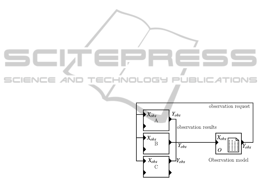
In DEVS, the solution generally used is to connect

models, both inputs and outputs, to an observation

model (see ﬁgure 2). This model has in charge to send

observation messages and to process the responses of

the models. For example, to build a discrete obser-

vation, the observation model relies on a constant ta

function in order to send, at each time step, an event

to observed models. Observed models compute ob-

servations values and send them to the observer.

Figure 2: This picture shows the classic observation mech-

anism to observe models in the DEVS formalism. Three

atomic models A, B and C are observed by an observation

model O which sends event for request observation on out-

put Y

obs

and waits the results on input port X

obs

in order to

store it in output ﬁles or databases.

This solution forces the modelers to merge the

state graphs between observation and behavior of

their models (See ﬁgure 3 for an explanation).

In addition, by merging the state graphs, the mod-

eler might make the results of its models dependent to

his observation. If model is observed asynchronously

with its behavior, the computation of the elapsed time

e when an external event disturbs an atomic model

may introduce a ﬂoating-point error. Indeed, coordi-

nator needs to call the external transition of the simu-

lator with s,e,x parameters where e = t −tl with t the

SIMULTECH2012-2ndInternationalConferenceonSimulationandModelingMethodologies,Technologiesand

Applications

init

Obs

init

Obs

Adding of

the capacity

to observe

the model

Figure 3: This picture show state graphs of an atomic model. In left picture, we show the model without observation and in

the right part, the same model with the capacity to be observed at any time (dotted lines represent external transitions). In

the computation of the observation states Obs

init

, Obs

or Obs

(in δ

ext

, δ

int

, δ

conf

or ta functions), simulators can introduce

ﬂoating-point errors when computing the time elapsed since last transition (e in DEVS terminology) for example.

current time of the simulation (time of the perturba-

tion) and tl the time of last event. If an internal state

variable in S is based on e to compute its value in the

ext

transition, its internal state variables can give dif-

ferent results with or without observations. Precisely,

this mismatch can be explained by the difﬁculty rep-

resenting real number in computer engineering (Gold-

berg, 1991) (see the IEEE Standard for Floating-Point

Arithmetic, IEEE 754).

If all models use integer as representation of the

time (i.e. all time advance functions return duration in

N), the ﬂoating-point problem would not exist. How-

ever, in the domain of Environmental Modeling, the

models use continuous and discrete event formalisms

such as the QSS2 formalism (Kofman, 2002) which

solves in R a second order polynomial function in

order to compute the duration in a state. They can

hardly rely on a representation of the time in N.

The solution proposed does not change the value

of e in the case of observation.

Finally, in DEVS, a model can have several states

at the same date (when at least one call to the ta(s)

function returns 0). These states are called transitory

states. It seems obvious that the observation of the

transitory states makes no sense. However, this solu-

tion does not guarantee to provide only observations

of real model states. For example, if the observation

is required at a speciﬁc time of simulation, the state

observed can be one of these transitory states.

In this section, we propose a formal and opera-

tional representation of observations in the PDEVS

formalism. This extension is based on a function of

observation in atomic models and a second graph of

connections in coupled models. This extension to the

PDEVS formalism integrates necessary characteris-

tics:

• First is to ensure that this extension does not dis-

turb the simulation i.e. we need to conserve the

same result with or without the observation.

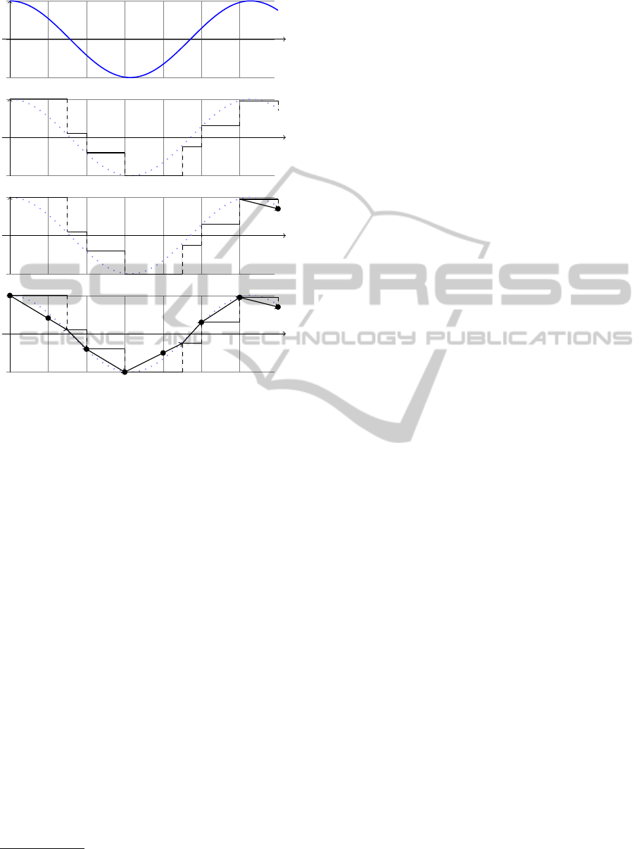
• Second is to provide several types of observation.

We propose, in this paper, two modes: time step

and ﬁnish that deﬁne respectively: observations

when a model reaches a time and observations at

the end of the simulation (see ﬁgure 4).

• Third, the extension should not take its values di-

rectly from the state of the current model but from

a function (see ﬁgure 4).

• Finally, in DEVS, state variables may change sev-

eral times at the same date (when its ta returns 0

or when an external event disturb it). In this case,

we observe the last state of the model.

Thus, to develop this extension we need to add

function to the atomic models, to add new set in cou-

pled model and add speciﬁc observation models. We

develop these changes in the next section.

2.2.1 PDEVS Atomic Model

To develop this extension in the PDEVS formalism,

we extend the PDEVS atomic model with new sets of

input and output ports (X

obs?

and Y

obs

). The ﬁrst one

is used for observation request; the second one is used

for routing values returned by modeler. We attach to

this port a new output function called λ

obs

. The new

PDEVS atomic model is deﬁned such as:

M = hX,Y,S,X

obs?

obs

,δ

int

,δ

ext

,δ

con

,λ, λ

obs

,tai

Where:

obs?

are the ports used to catch

observation requests.

obs

are the ports used to send observation values.

ObservationsofDiscreteEventModels

State of a system

DEVS transitory state

Finish observation

Timed observation

Figure 4: The ﬁrst ﬁgure shows the evolution of the state S

of a system over time t. The second ﬁgure shows the model

of this system in DEVS. This ﬁgure shows the trajectory of

the state of the DEVS model. The last two ﬁgures show the

extension observation described in this paper in time-step

(∆

= 1) or in ﬁnish mode. This extension allows the mod-

eler to provide a function (observation) that computes an

observation value. Dots are observation values. These val-

ues are computed by interpolation of the current DEVS state

of s and e, the elapsed time since the last transition.

obs

: X

obs?

× s ×t

obs

→ Y

obs

s ∈ S,

obs

current time of the simulation.

This deﬁnition allows us to represent both

observed models and classical PDEVS models

as deﬁned in section 2.1. Indeed, the model

hX,Y,S, X

obs?

obs

,δ

int

,δ

ext

,δ

con

,λ, λ

obs

,tai with no

observations

is equivalent to the classical PDEVS

atomic model hX,Y, S,δ

int

,δ

ext

,δ

con

,λ, tai. In fact,

we should distinguish observed models from observer

models.

2.2.2 Observer Models

In this paper, we suggest two types of observers.

timed

, and O

ﬁnish

to respectively, send observation

following a given time-step or at the end of the simu-

lation.

obs?

0, Y

obs

0 and λ

obs

is a null function.

• The discrete time observer model, O

timed

, needs

to send output events on its output port Y

obs

every

∆

unit time. O

timed

reads observation events from

its port X

obs

and stores data transported by event.

This model is :

timed

= hX

obs

obs?

,S, X

obs?

obs

int

,δ

ext

,δ

con

,λ, λ

obs

,tai

Where:

obs

is the set of observation values,

obs?

is the set of observation requests,

S : {IDLE,SENT} × Data, with:

IDLE, SENT: automata ﬁnite states,

Data: output stream states.

obs?

obs

∀d ∈ Data : δ

int

((IDLE, d)) = (SENT,d)

∀d ∈ Data : δ

int

((SENT, d)) = (IDLE,d)

∀s ∈ {IDLE,SENT } :

ext

((s,d),e,X

obs

) = (s, d

)

where d

is the state of the output stream

once X

obs

has been stored,

∀d ∈ Data : ta((IDLE, d)) = ∆

(the time step)

∀d ∈ Data : ta((SENT, d)) = 0

∀s ∈ S : λ(s) = observation(s,t,x)

obs

is a null function

• The ﬁnish observer model, O

ﬁnish

, produces ob-

servation events at the end of the simulation on it

obs

port and wait observation events from its port

obs

. O

ﬁnish

is the same model as O

timed

but, its ta

function returns the end of the simulation to build

observation event, or +∞ after.

timed

= hX

obs

obs?

,S, X

obs?

obs

int

,δ

ext

,δ

con

,λ, λ

obs

,tai

Where:

obs

is the set of observation values,

obs?

is the set of observation requests,

S : {WAIT,END} × Data, with:

WAIT, END: automata ﬁnite states,

Data: output stream states.

∀d ∈ Data : δ

int

((WAIT, d)) = (END, d)

∀d ∈ Data : δ

int

((END,d)) = (END,d)

∀s ∈ {WAIT,END} :

ext

((s,d),e,X

obs

) = (s, d

)

SIMULTECH2012-2ndInternationalConferenceonSimulationandModelingMethodologies,Technologiesand

Applications

where d

is the state of the output stream

once X

obs

has been stored,

obs?

obs

∀d ∈ Data : ta((WAIT,d)) = end

where end is the duration of simulation

∀d ∈ Data : ta((END,d)) = +∞

∀s ∈ S : λ(s) = observation(s,t,x)

obs

is a null function

The function observation is a user deﬁned func-

tion that identiﬁes in Y

obs?

the observation request that

should be sent to the observed models.

2.2.3 Coupled Model

As seen earlier in the introduction and in the section

2.1, the I

variable and the function Z

i,d

deﬁne the

graph of connections of the models by calculating the

inﬂuenced models. Our observation extension of the

PDEVS formalism uses the same principle. It pro-

poses two subsets I

and I

that, respectively iden-

tify the inﬂuences of atomic models (responses of the

observations) and the inﬂuences of observer models

(models sending the request of observation).

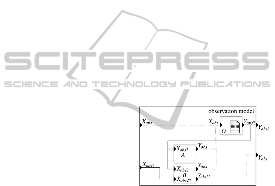
We extend the PDEVS model coupled in order to

introduce a second connection network (see the ﬁgure

5). This second network is dedicated to the observer

models and to the classical PDEVS atomic models to

observe through their ports X

obs?

and Y

obs

. The new

PDEVS coupled model is deﬁned as:

N = hX,Y,D, O,R,X

obs?

obs

obs?

obs

},{I

},{Z

i,d

},{O

},{Z

o,d

},{M

},{R

},{Z

r,d

Where X

obs

, Y

obs

and X

obs?

, Y

obs?

are input and out-

put ports to route observation and request events. O

is the set of names of observed models O ⊆ D, {M

}

is the set of observed models {M

} ⊆ {M

} , R is the

set of names of observer models R ⊆ D and {M

} is

the set of observer models {M

} ⊆ {M

∀r ∈ R ∪ {N},

is the inﬂuencer set of observed models of r

⊆ O ∪ {N},r /∈ I

∀o ∈ O ∪ {N},

is the inﬂuencer set of observed models of o

⊆ R ∪ {N},o /∈ I

The observation network is however very con-

strained. Thus, the functions Z

o,d

and Z

r,d

are very

different and provide additional constraints from the

classical Z

i,d

function. These additional constraints

ensure that a DEVS atomic model cannot send an ob-

servation event to another DEVS atomic model, and

an observation model cannot send request observa-

tion to another observation model. The ﬁgure 5 shows

an example of connections between observed and ob-

server models.

∀r ∈ R ∪ {N},

∀d ∈ I

,∃ an output translation function Z

r,d

: X

obs?

→ X

obs?

, if r = N

r,d

: Y

obs?

→ Y

obs?

, if d = N

r,d

: Y

obs?

→ X

obs?

, if r 6= N and d 6= N

∀o ∈ O ∪ {N},

∀d ∈ I

,∃ an output translation function Z

o,d

: X

obs

→ X

obs

, if o = N

o,d

: Y

obs

→ Y

obs

, if d = N

o,d

: Y

obs

→ X

obs

, if o 6= N and d 6= N

Figure 5: In this picture, we illustrate the second network

in the coupled model to deal with observations graph. Plain

connections are observation requests from output port Y

obs?

of observation models, to atomic model input port X

obs?

to coupled model’s output port Y

obs?

, or from coupled model

input port X

obs?

to atomic model X

obs?

. Dashed connections

constitute response of observation request from extended

PDEVS atomic model (on output port Y

obs

) to observation

model X

obs

or coupled model output port Y

obs

. The atomic

model B is observed by an external observation model on

its port X

obs2

. It sends observations to its output port Y

obs2

For this ﬁgure and for a better understanding, we distinguish

observation ports for the model B.

2.2.4 Closure Under Coupling

Since we keep unchanged the internal S of coupled

or atomic models nor all sets of the PDEVS deﬁni-

tion (IMM, INF(s), CONF(s), EXT(s) and UN(s) of

ObservationsofDiscreteEventModels

Listing 1: Root coordinator algorithms.

Parallel−Devs−Root−Coordinator

variables:

t // current simulation time

child // direct subordinate devs−simulator

// or devs−coordinator

t = t

send initialization message (i,t) to child

t = tn of its child

loop

send (∗,t) message to child

t = tn of its child

until end of simulation

end Parallel−Devs−Root−Coordinator

the coupled model), the PDEVS functions have the

same content (See chapter 7 in (Zeigler et al., 2000) to

the complete formalization). The closure under cou-

pling property of the extension observation for paral-

lel DEVS is still veriﬁed.

2.3 Algorithms

2.3.1 Root Coordinator

The root-coordinator implements the overall simula-

tion loop. It sends messages to its direct subordi-

nate (simulator or coordinator). The root-coordinator

ﬁrst sends an initialize message (i-message), and loop

on internal transition (*-message) from its child to

perform the simulation cycles until some termination

conditions.

As describe in the listing 1, the root coordinator is

unchanged in this extension.

2.3.2 Coordinator

In the coordinator algorithm, we add an additional

variable tb, which indicates the last date of the sim-

ulation. This variable tb detects the last PDEVS bags

to ensure to observe the latest state of a model. We

add a new bag, called mailobs to store all observation

events to atomic models at a speciﬁc date. When tb

detect a change, the mailobs is ﬂushed into the obser-

vation network using the functions Z

r,d

and Z

o,d

The coordinator’s algorithms are described in the

listings 2. From l. 1 to l. 38: routes the message or

stores in mailobs. From l. 40 to the end: to update the

tb variable and to send xobs?-message to the atomic

models.

Listing 2: Coordinator algorithms.

1 Parallel−Devs−Coordinator

2 variables:

3 DEVN = (X, Y , D, {M

}, {I

}, {Z

i,d

})

4 parent // parent coordinator

5 tl // time of last event

6 tn // time of next event

7 eventlist // list of element (d, tn

) sorted by tn

8 mail // output mail bag

9 mailobs // observation mail bag

10 O

event

// event−list of event observation model

11 y

parent

// output message bag to parent

12 y

// set of output message bags for each child d

14 when receive xobs−message (x

obs

,t)

15 if not (tl ≤ t ≤ tn) then

16 error: bad synchronisation

17 receivers = {o|o ∈ children,o ∈ I

}

18 for each o ∈ receivers

19 send x−message (Z

r,d

(x) with input value Z

r,d

to o

21 when receive xobs?−message (x

obs?

,t)

22 if not (tl ≤ t ≤ tn) then

23 error: bad synchronisation

24 receivers = {r|r ∈ children,r ∈ I

}

25 for each r ∈ receivers

26 add r, x

obs?

to mailobs

28 when receive yobs−message (y

obs

,t) from o

29 for each child d ∈ Z

o,d

30 send xobs−message to d

31 for each d ∈ Z

o,d

and d = N

32 send yobs−message to parent

34 when receive yobs?−message (y

obs?

,t) from r

35 for each child d ∈ Z

r,d

36 send yobs−message to d

37 for each d ∈ Z

r,d

and d = N

38 send yobs?−message to parent

40 // ﬁnally, we append these algorithms

41 // in the following message

43 when receive i−message (i,t) at time t

44 [...] // The same algorithms than PDEVS

45 tb = tl

47 when receive ∗−message, x−message or y−mess

48 age

49 if tb != t then

50 for each r, x

obs?

∈ mailobs

51 send xobs?−message (Z

r,tb

(x) with

52 input value Z

r,d

to r

53 mailobs =

54 tb = t

55 [...] // The same algorithms than PDEVS

57 end Parallel−Devs−Coordinator

SIMULTECH2012-2ndInternationalConferenceonSimulationandModelingMethodologies,Technologiesand

Applications

Listing 3: Simulator algorithms.

1Parallel−Devs−Simulator

2variables:

3parent // parent coordinator

4tl // time of last event

5tn // time of next event

6DEV S // associated model with total state (s,e)

obs

// output observation bag

9// The same algorithms than PDEVS simulator

10// see chapter 11

11[...]

13when receive xobs?−message (x

obs?

,t) at t

14with input x

obs?

15y

obs

= λ

obs

obs?

,t)

16send yobs−message (y

obs

,t) to parent coordinator

18end Parallel−Devs−Simulator

2.3.3 Simulator

Lastly, this last section on the abstract simulators

develops algorithm for the simulator of the atomic

model. As presented previously, the management of

the observations events is very simple for the modeler

since only one function is called λ

obs

. This function

is called only for classical atomic models when they

receive an X

obs?

event. When observation models re-

ceives X

obs

event, they use the classical way when re-

ceiving input message (See x-message in PDEVS ab-

stract simulators).

The listing 3 describes the simulators algorithms.

In line 12: when receives an xobs?-message from the

parent, simulator computes the observation in the λ

obs

function and sends the data (wrapped into an yobs-

message) to the parent coordinator.

To validate this work, we made an implementation

of this extension in the DEVS open source simulator

VLE.

3 RESULT

These works have started with multi-disciplinary is-

sues emerging from the interaction between computer

scientists and biologists. Considering these works,

we think that the integration of heterogeneous models

and the respect of the M&S cycle are the key issues to

provide a complete and reliable software environment

for natural complex systems modeling. Therefore,

VLE has evolved on a complete multi-modeling and

simulation environment (Quesnel et al., 2009) and is

now a generic environment for M&S, in Environmen-

tal Sciences, in Industry or Medicine. Many projects

from two major French research institutes INRA and

Cirad use VLE. For example, the RECORD project

(Bergez et al., 2012) is a large platform designed for

developing and analyzing models of cropping sys-

tems.

3.1 VLE: Virtual Laboratory

Environment

VLE is a set of programs and libraries software.

These components are used to model, to simulate and

to analyze multimodel. VLE offers a set of formalism

developed with a DEVS BUS (Kim and Kim, 1996).

The sub-formalisms are DESS, QSS 1 and QSS 2

numerical procedure for solving ordinary differential

equations, Petri nets, ﬁnite state automaton (moore,

mealy, FDDEVS and Harel statechart (Harel, 1987)),

cellular automaton (Cell-DEVS and Cell-QSS) and

agent decision making. These extensions are devel-

oped using a DEVS BUS i.e. these extensions are de-

veloped such as atomic model. Finally, VLE uses an

open-source license and all the source code are avail-

able on its website including this observation exten-

sion.

DEVS BUS

• Scheduller,

• Network.

Simulator

Petrinet

Simulator

QSS 2

(x, t)

(y, t)

(∗, t)

(done, tN)

Figure 6: DEVS BUS and multi-modeling. The events

(x,t), (y,t), (∗,t), (done,tN) represent the bus.

3.2 Implementation

In our implementation of the PDEVS abstract simu-

lator, we deﬁne an atomic model as a classical C++

class. Modeler must this class inherits this class to

override the observation function and to beneﬁt to the

observation extension developed in the previous sec-

tion

The listing 4 shows a simpliﬁed representation

(without constructor, destructor, and other members)

of the class which permits to develop atomic model

behavior:

• l. 3-14: the classic PDEVS functions: ta, δ

int

, δ

ext

λ and δ

con

• l. 15: the observation method is called when an

observation event arrived on a input observation

ObservationsofDiscreteEventModels

Listing 4: The C++ interface of the simulators in VLE.

1class Dynamics {

2public:

3virtual Time timeAdvance() const;

4virtual void internalTransition(

5const Time& time);

6virtual void externalTransition(

7const Time& time,

8const ExternalEventList& lst);

9virtual void output(

10const Time& time,

11ExternalEventList& out) const;

12virtual void confluentTransition(

13const Time& time,

14const ExternalEventList& lst);

15virtual Value* observation(

16const ObservationEvent& event) const;

17};

port X

obs

. λ

obs

is also a constant function to pre-

vent user to modify the state of its model. This

function returns a Value (simple type as integer,

real, Boolean, string, and complex type as set, dic-

tionary, matrix.).

Thus, the observation function of the simulator

that implements the Euler method (a numerical pro-

cedure for solving ordinary differential equations) in

VLE, the C++ code is:

1 Value* Euler::observation(

2 const ObservationEvent& event) const

3 {

4 double e = event.getTime() - mLastTime;

6 return getEstimatedValue(e);

7 }

The function getEstimatedValue calculates an

approximation of the value of the variable. It uses

the current value of the state variable and the time

elapsed since the last transition. This observation

function does not change the current state of the vari-

able. Thus, we respect the reproducibility of the sim-

ulation. However, we create additional cost calcu-

lations for each observation. This extra cost can be

important if the observation function is complex and

if called often. However, we believe that observing

a model often is only needed when debugging the

model.

3.3 Using Models with VLE

The study of the models is very important in the mod-

eling and simulation cycle. Generally, this analysis is

performed with an experimental setting. Experimen-

tal frames as sensitivity analysis, replicas generation

are used to study or to validate models. One impor-

tant motivation in formalizing the observation process

in PDEVS is to develop generic experimental frames,

which ones rely on intensive observation of models.

VLE is an environment for M&S. It relies on a

set of libraries for modeling, simulation and analy-

sis. These libraries developed in C++ are available

for several programming languages. Thus, in order

to collaborate with users of statistical tools, we pro-

vide an interface to the program R (R Development

Core Team, 2012). R is a tool and language for statis-

tical computing. This package named RVLE allows

the user to run simulations, changes its parameters

and retrieves simulation results (from the extension

observation). This package combined with another

packages of R as the classical sensitity package per-

mit to build experimental frames to validate, explore

and optimize models. On this principle, we also offer

program and PYVLE JVLE to develop web services

based on simulation.

4 CONCLUSIONS

In this paper, in section 2, we extend the PDEVS for-

malism to introduce the observation of models in the

formalism. This work was motivated by the separa-

tion between the dynamics of the system and its ob-

servation as a fundamental issue. This addition to the

formalism is closed under coupling and allows build-

ing observations in a hierarchical and modular man-

ner. The abstract simulators necessary for this exten-

sion were provided. In addition, we provided an im-

plementation of this observation extension in the VLE

simulators. This DEVS extension is crucial for us to

develop experimental design and to abstract observa-

tion from models dynamic. However, a type of obser-

vation is missing in these works. It concerns the event

observation of atomic models. In PDEVS terminol-

ogy, after each change in δ

int

, δ

ext

or δ

con

transition

functions. We work on the formalization of this new

type of observation.

REFERENCES

Bergero, F. and Kofman, E. (2010). PowerDEVS: a tool

for hybrid system modeling and real-time simulation.

SIMULATION.

Bergez, J.-E., Chabrier, P., Gary, C., Jeuffroy, M.,

Makowski, D., Quesnel, G., Ramat, E., Raynal, H.,

Rousse, N., Wallach, D., Debaeke, P., Durand, P.,

Duru, M., Dury, J., Faverdin, P., Gascuel-Odoux, C.,

and Garcia, F. (2012). An open platform to build, eval-

uate and simulate integrated models of farming and

SIMULTECH2012-2ndInternationalConferenceonSimulationandModelingMethodologies,Technologiesand

Applications

agro-ecosystems. Environmental Modelling And Soft-

ware. In press.

Chow, A. and Zeigler, B. (1994). Parallel DEVS: a parallel,

hierarchical, modular, modeling formalism. In Pro-

ceedings of the 26th conference on Winter simulation,

pages 716–722, Orlando, Florida, United States.

Goldberg, D. (1991). What every computer scientist should

know about ﬂoating-point arithmetic. ACM Comput-

ing Surveys, 23:5–48.

Harel, D. (1987). Statecharts: A visual formalism for com-

plex systems. Sci. Comput. Program., 8:231–274.

Himmelspach, J. and Uhrmacher, A. M. (2009). The

JAMES II Framework for Modeling and Simula-

tion. In International Workshop on High Performance

Computational Systems Biology, pages 101–102.

Kim, Y. J. and Kim, T. G. (1996). A heterogeneous dis-

tributed simulation framework based on DEVS for-

malism. In Sixth Annual Conference On Artiﬁcial In-

telligence, Simulation and Planning in High Auton-

omy Systems, pages 116–121, La Jolla, California,

USA.

Kofman, E. (2002). A second order approximation for devs

simulation of continuous systems. Simulation (Jour-

nal of The Society for Computer Simulation Interna-

tional, 78(2):76–89.

Quesnel, G., Duboz, R., and Ramat, E. (2009). The Virtual

Laboratory Environment – An operational framework

for multi-modelling, simulation and analysis of com-

plex dynamical systems. Simulation Modelling Prac-

tice and Theory, 17:641–653.

R Development Core Team (2012). R: A Language and

Environment for Statistical Computing. R Foundation

for Statistical Computing, Vienna, Austria. ISBN 3-

900051-07-0.

Ribault, J., Dalle, O., Conan, D., and Leriche, S. (2010).

OSIF: a framework to instrument, validate, and ana-

lyze simulations. In SIMUTools ’10 Proceedings of

the 3rd International ICST Conference on Simulation

Tools and Techniques.

Vangheluwe, H. (2000). DEVS as a common denominator

for hybrid systems modelling. In Varga, A., editor,

IEEE International Symposium on Computer-Aided

Control System Design, pages 129–134, Anchorage,

Alaska. IEEE Computer Society Press.

Zeigler, B. P., Kim, D., and Praehofer, H. (2000). Theory of

modeling and simulation: Integrating Discrete Event

and Continuous Complex Dynamic Systems. Aca-

demic Press.

ObservationsofDiscreteEventModels