
Machine Modelling for Transient Stability Analysis
in Distribution Grids
A Comparison of Synchronous and Induction Machine Models in Medium
and Low Voltage Grids
Johannes Weidner and Lutz Hofmann
Institute of Electric Power Systems, Leibniz University Hannover, Appelstraße 9a, Hannover, Germany
Keywords: Transient Stability, Distribution Grid, Machine Modelling, Distributed Generation.
Abstract: The complete models for synchronous and induction machines are compared with selected approximated
models. This is to validate the approximations for the utilisation in transient stability analysis in distribution
grids. The results show that they can be used to simulate stable oscillations, but they lose their accuracy
approaching the area of transient instability. The main reason is the active power exchange during faults,
which is not jumping to zero as it does in high voltage scenarios.
1 INTRODUCTION
The installed power of distributed generation units in
the medium and low voltage grids is continuously
increasing. Substituting conventional technologies,
reliability and stability of these units has to increase
proportional. Therefore the consequences to the
stability in the resulting weakly meshed multi
machine systems have to be analysed. This is not a
standard procedure, since resistances of the grid
cannot be neglected as in the high voltage grid.
Additional the machine parameters can have
different relations to each other.
This paper is focused on the modelling of
rotating machines in distribution grids under the
perspective of transient stability analysis. This is
done by comparing complete models for
synchronous and induction machine with selected
approximated models. The approximated models are
equivalent to the standard transient model of
synchronous machines (Kundur, 2007). These
models are easy to use in initialisation and
simulation, because they can be reduced to a
mechanical equation system and an equivalent
circuit with constant voltage source.
The aim is to validate these alternative models
also for the utilization in transient stability analysis
regarding distribution grids.
2 SIMULATION MODEL
The analysis is based on a simulation model, which
is suitable for meshed grids. The equation system is
taken from the literature and then modified to
receive an approximated model with comparable
parameters and variables. In this paper a simple test
grid with one machine and its connection to the
overlaying grid will be used to obtain a qualitative
comparison of the investigated machine models. The
scenario for the transient stability analysis assumes a
3-phase fault in the overlaying grid N, which the
generator G should run through without transient
instability.
Figure 1: Topology of the basic scenario.
The complete model of the synchronous machine
is taken from the literature. Other models were
derived from the corresponding equation system to
receive a formulation with similar parameters and
variables. The natural behavior of the machine
models is analyzed, so the excitation and the
367
Weidner J. and Hofmann L..
Machine Modelling for Transient Stability Analysis in Distribution Grids - A Comparison of Synchronous and Induction Machine Models in Medium and
Low Voltage Grids.
DOI: 10.5220/0004055603670376
In Proceedings of the 2nd International Conference on Simulation and Modeling Methodologies, Technologies and Applications (SIMULTECH-2012),
pages 367-376
ISBN: 978-989-8565-20-4
Copyright
c
2012 SCITEPRESS (Science and Technology Publications, Lda.)

mechanical torque were held constant during the
simulations.
As component parameters typical values for
voltage level and rated power were chosen. The
rated parameters for the scenarios are listed below.
Table 1: Rated parameters for the scenarios.
Parameter Medium Voltage Low Voltage
N
U
110 kV 20 kV
S
k,N
6 GVA 0,5 GVA
T1
S
40 MVA 630 kVA
L
3 km 300 m
type
AL/ST 3x50/8/20 NAYY 4x120/0
T2
S
2 MVA
-
G
U
600 V 400 V
S
2 MVA 100 kVA
2.1 Electrical Grid
Due to the relatively small voltage in distribution
grids the line capacities have only a small effect on
the load flow and can be neglected for transient
stability analysis.
The model is following the extended nodal
method (Oswald, 2009) for resistive and inductive
grids. Voltages and currents are formulated as space
phasors g
which can be transformed from and to the
momentary values of each phase g
a
, g
b
and g
c
, using
the complex phasor a
=0,5 -1+j
√
3.
g
=
g
r
g
r
*
g
h
=
2
3
1a
a
2
1a
2
a
11 1
g
a
g
b
g
c
(1)
All grid components, like transformers, lines and
machines, consist of a reactance R
L
, an inductance
L
L
and a voltage source
u
qL
connected in series.
Please note that considering the phase shifting of
transformers
L
L
can be complex.
u
L
=R
L
i
L
+L
L
i
L
+u
qL
(2)
The connection between components and nodes
is described by a coupling matrix K
LL
. An algebraic
equation is used to calculate the nodal voltages
u
L,all
from the currents i
L,all
and voltage sources u
qL,all
, as
vectors of all the components phasors.
u
L,all
=-K
LL
T
K
LL
L
L,all
-1
K
LL
T
-1
K
LL
L
L,all
-1
∙
R
L,all
i
L,all
+u
qL,all
(3)
The voltage sources are either defined by the
input data or calculated from the state variables of
the components.
2.1.1 Complete Model
In the complete model the currents of inductances
are state variables. From the voltage equation of
each component, the differential equation for the
currents can easily be obtained.
i
L
=L
L
-1
u
L
−R
L
i
L
−u
qL
(4)
2.1.2 Approximated Model
The state variables of the grid can be assumed as
steady state. In this case voltages and currents are
sinusoidal with a constant grid frequency ω
N
. In the
formulation with rotating space phasors the
derivative is imaginable as the tangent at the point of
operation. For balanced conditions the space phasor
is moving in a circle.
i
L
=jω
N
i
L
=
j00
0-j0
000
ω
N
i
L
(5)
This leads to the formulation with complex
impedances for the resistive and inductive branch.
u
L
=
+jω
N
·L
L
i
L
+u
qL
(6)
Because the nodal voltages u
L,all
can be
calculated from currents i
L,all
and voltage sources
u
qL,all
, the equations can be transposed to the steady
state currents. Doing so a current depending part ΔZ
of the voltage source has to be taken into account.
u
qL
=ΔZ i
L
+u
qL
(7)
i
L,all
=−jω
N
L
L,all
+
,
+ΔZ
∙u
q
L,all
(8)
=K
LL
T
K
LL
L
L,all
-1
K
LL
T
-1
K
LL
L
L,all
-1
+
(9)
2.1.3 Simulation Parameters
The parameters are chosen to represent typical grid
scenarios for a medium and a low voltage feed in,
neglecting the parallel strings in a radial grid.
SIMULTECH2012-2ndInternationalConferenceonSimulationandModelingMethodologies,Technologiesand
Applications
368

Table 2: Simulation parameters for the grid components
referred to the nominal voltage of the considered grid.
Parameter
Medium Voltage Low Voltage
R
N
0 Ω 0 Ω
L
N
0,23 mH 1,1μH
R
25 mΩ 13,5 mΩ
L
3,5 mH 2,8 mH
R
1,7 Ω 0,25 Ω
L
3,5 mH 0,31 mH
R
1,5 Ω
-
L
41 mH
-
2.2 Synchronous Machine (SM)
Synchronous machines are used in conventional
power plants. Therefor a lot of models and analysis
on their transient behaviour in high voltage grids
exist. In distribution grids they are used to connect
plants which operate with constant shaft frequency.
The model of the synchronous machine is made
up of a resistance R
L
, an inductance L
L
and a
controlled voltage source u
qL
connected in series.
2.2.1 Complete Model (SMc)
The equation system of the resistance the
inductance, the controlled voltage source and the
inner states of the machine is taken from (Hofmann,
2003). The considered eight state variables are:
the three stator currents i
L
, modelled as
rotating space phasors,
the rotor flux linkages of the excitation
winding Ψ
F
as well as of the damping winding
in the d-axis Ψ
D
and in the q-axis Ψ
Q
,
the angular frequency ω
LF
and
the angle of the rotor ϑ
LF
.
The equations related to the coupling with the
grid are written below. A magnetic saliency
(L
d
''
≠L
q
''
) causes angle depending elements in the
resistance and the inductance matrices.
R
L
=
R
a
jω
LF
−
e
-2jϑ
LF
0
-jω
LF
−
e
2jϑ
LF
R
a
0
00R
0
(10)
L
L
=
1
2
L
d
''
+L
q
''
−
e
-2jϑ
LF
0
−
e
2jϑ
LF
L
d
''
+L
q
''
0
002L
0
(11)
u
qL
≈
e
jϑ
LF
00
0e
-jϑ
LF
0
001
ω
LF
jj-1
-j -j -1
000
-
H
FF
+H
DF
H
DD
+H
FD
jH
QQ
H
FF
+H
DF
H
DD
+H
FD
-jH
QQ
000
k
F
Ψ
F
k
D
Ψ
D
k
Q
Ψ
Q
(12)
The additional small effects of stator currents
and excitation voltage on the voltage source are not
shown in the equation.
The behaviour of the inner state variables is
characterised by a differential equation system,
using the Park-transformation for the stator currents.
i
d
i
q
i
0
=
1
2
110
-j j 0
002
e
-jϑ
LF
00
0e
jϑ
LF
0
001
i
L
(13)
k
F
Ψ
F
k
D
Ψ
D
k
Q
Ψ
Q
= −
H
FF
H
FD
0
H
DF
H
DD
0
00H
QQ
k
F
Ψ
F
k
D
Ψ
D
k
Q
Ψ
Q
+
k
F
2
R
F
00
k
D
2
R
D
00
0 k
Q
2
R
Q
0
i
d
i
q
i
0
+
k
F
u
F
0
0
(14)
m
e
=
3p
2
L
d
''
-L
q
''
i
d
i
q
+
+
−
(15)
ϑ
LF
=
00
10
ω
LF
ϑ
LF
+
+
0
(16)
The behavior of the machine is influenced by the
turbine torque on the rotor shaft m
m
and the
excitation voltage u
F
, which are both considered
constant in this model.
2.2.2 Approximated Model (SMa)
In the conventional model for transient analysis the
stator currents and the d-axis currents in the
damping winding are considered to be steady state.
This leads to a separation of the voltage source u
qL
in a inductive part Δ
L
' and a transient voltage u
qL
'
,
which is considered to have a constant amplitude.
u
L
=u
qL
'
+
R
L
+jω
LF
L
L
+jω
LF
ΔL'
i
L
(17)
Similar results can be obtained when the q-axis
currents in the damping winding are also considered
to be steady state. This leads to the advantage that
the magnetic saliency can still be taken into account.
MachineModellingforTransientStabilityAnalysisinDistributionGrids-AComparisonofSynchronousandInduction
MachineModelsinMediumandLowVoltageGrids
369

ΔL'=
1
2
ΔL
d
'
+ΔL
q
'
ΔL
d
'
-ΔL
q
'
e
-2jϑ
LF
0
ΔL
d
'
-ΔL
q
'
e
2jϑ
LF
ΔL
d
'
+ΔL
q
'
0
000
(18)
ΔL
d
'
=
k
D
2
R
D
H
DD
(19)
ΔL
q
'
=
k
Q
2
R
Q
H
(20)
The transient voltage is constant when the rotor
frequency and the flux linkages of the excitation
winding do not change.
u
qL
'
≈ H
DD
H
FF
-H
DF
H
FD
1
1
0
−jω
LF
H
DD
-H
DF
1
-1
0
k
F
Ψ
F
0
H
DD
(21)
The differential equation of the rotor flux
linkages is substituted by an algebraic equation,
depending on the stator currents and its initial
value Ψ
F
.
k
F
Ψ
F
k
D
Ψ
D
k
Q
Ψ
Q
=
1
-H
DF
H
DD
0
k
F
Ψ
F
+
00
ΔL
d
'
0
0 ΔL
q
'
i
d
i
q
(22)
Due to this constant flux linkage the number of
state variables could be reduced to two variables.
The differential equations of rotor frequency and
rotor angle are not directly changed, but the equation
of the flux linkages can be inserted.
m
e
=
3p
2
∙L
d
''
+ΔL
d
'
-L
q
''
-ΔL
q
'
·i
d
i
q
+1−
∙
∙
(23)
2.2.3 Simulation Parameters
The parameters are chosen to represent typical
values for synchronous machines with the
designated rated power and voltage.
Table 3: Parameters for the synchronous generator
referred to the nominal voltage of the considered grid.
Parameter
Medium
Voltage
Low Voltage
R
a
2,2 Ω 57 mΩ
L
d
''
73 mH 0,55 mH
L
q
''
0,11 H 0,96 mH
H
FF
2,9 s
-1
22 s
-1
H
DF
-41 s
-1
-61 s
-1
H
FD
-2,7 s
-1
-22 s
-1
H
DD
43 s
-1
64 s
-1
H
QQ
8,3 s
-1
20 s
-1
R
F
0,53 Ω 22 mΩ
R
D
8,1 Ω 64 mΩ
R
Q
9,0 Ω 0,15 Ω
k
F
0,60 0,38
k
D
0,37 0,60
k
Q
0,86 0,82
p
2 2
J
57 kgm
2
1,1 kgm
2
2.3 Induction Machine (IM)
Besides inverters, where the transient behaviour can
be chosen within the current and voltage limits, most
of the generation units in distribution grids are
connected to the grid via induction machines.
The models used in this paper are derived from
the presented complete model of the synchronous
machine. Therefore the excitation winding was
extracted, the magnetic saliency was neglected and
an excitation voltage for the remaining rotor winding
was implemented (u
and u
Q
). In steady sate
operations this voltages are impressed with the slip
frequency of the rotor.
2.3.1 Complete Model (IMc)
The model considers seven state variables:
the three stator currents i
L
, modelled as
rotating space,
the rotor flux linkages of the rotor winding in
the d-axis Ψ
D
and in the q-axis Ψ
Q
,
the angular frequency ω
LF
and
the angle of the rotor ϑ
LF
.
Please note that the state variables can be
reduced by the angle rotor, when there is no
excitation voltage, or an excitation voltage which is
always in phase with the rotor flux linkages.
SIMULTECH2012-2ndInternationalConferenceonSimulationandModelingMethodologies,Technologiesand
Applications
370

The equations related to the coupling with the
grid are relatively simple. This is caused by the
symmetrical windings.
R
L
=
R
a
00
0 R
a
0
00R
0
(24)
L
L
=
L
''
00
0 L
''
0
00L
0
(25)
u
qL
=
k
LF
2
R
LF
00
0 k
LF
2
R
LF
0
000
i
L
+
PRa
k
LF
u
d
k
LF
u
q
+
k
LF
T
LF
1+jω
LF
T
LF
00
01-jω
LF
T
LF
0
000
PRa
Ψ
D
Ψ
Q
(26)
The transformation matrix
PRa
, converts to the
space phasor representation.
PRa
=
e
jϑ
LF
0
0e
-jϑ
LF
00
1j
1-j
(27)
The behaviour of the inner state variables is
characterised by a differential equation system,
using the Park-transformation for the stator currents.
i
d
i
q
i
0
=
1
2
110
-jj0
002
e
-jϑ
LF
00
0e
jϑ
LF
0
001
·i
L
(28)
k
LF
Ψ
D
k
LF
Ψ
Q
=
k
LF
2
R
LF
00
0 k
LF
2
R
LF
0
i
d
i
q
i
0
−
1
T
LF
0
0
1
T
LF
k
LF
Ψ
D
k
LF
Ψ
Q
+
k
LF
u
D
k
LF
u
Q
(29)
m
e
=
3p
2
k
LF
Ψ
D
·i
q
-k
LF
Ψ
Q
·i
d
(30)
The equation of motion is similar to the
synchronous machine. Though, the behavior of the
machine is influenced by the mechanical torque on
the rotor shaft m
m
, which is considered to be
constant in this model, and the excitation voltages in
the rotor winding u
D
and u
, which are assumed to
rotate with slip frequency.
2.3.2 Approximated Model (IMa)
There is no classic model for the transient analysis
of induction machines. Both, the steady state and the
short circuit model are not suitable in any scenario.
Therefore an equivalent approach as for the
synchronous machine is implemented. In the first
step the stator currents are considered to be steady
state and in the second step the amplitude of the
rotor flux linkage Ψ is hold constant. This leads to a
model with three state variables ω
LF
, ϑ
LF
and ϑ
Ψ
,
where ϑ
Ψ
is the angle of the flux. The angles can be
again combined to one variable, when there is no
excitation voltage or when the excitation voltage is
perfectly in phase with the flux linkage.
Ψ
0
=Ψ
D
+jΨ
Q
(31)
ϑ
Ψ
=∠Ψ
D
+jΨ
Q
(32)
In the equivalent circuit on the grid side only the
formulation of the flux linkage in the voltage source
equation is changed.
k
LF
Ψ
D
k
LF
Ψ
Q
=k
LF
Ψ
0
∙
cos
ϑ
Ψ
sin
ϑ
Ψ
(33)
The differential equations of the inner state
variables are formulated using the equation system
of the complete machine model.
ϑ
Ψ
=
Ψ
Q
Ψ
0
cos
ϑ
Ψ
-
Ψ
D
Ψ
0
sin
ϑ
Ψ
(34)
m
e
=
3p
2
k
LF
Ψ
0
cos
ϑ
Ψ
i
q
-k
LF
Ψ
0
sin
ϑ
Ψ
i
d
(35)
2.3.3 Simulation Parameters
The parameters are chosen to represent typical
values of induction machines with the designated
rated power and voltage.
Table 4: Simulation parameters of the induction machine
referred to the nominal voltage of the considered grid.
Parameter Medium Voltage Low Voltage
R
a
1,0 Ω 0,18 Ω
L
''
0,13 H 0,76 mH
T
LF
2,0 s 0,56 s
R
LF
1,0 Ω 0,18 Ω
k
LF
0,97 0,96
p
2 3
J
108 kg
m
1,2
k
g
m
3 SHORT CIRCUIT SIMULATION
Both machines and their approximated models
where confronted with a short circuit in the
MachineModellingforTransientStabilityAnalysisinDistributionGrids-AComparisonofSynchronousandInduction
MachineModelsinMediumandLowVoltageGrids
371
overlaying grid. The aim is to compare the models
on the basis of their transient behaviors. As
explained below, the maximal amplitude of the
voltage source angles (referred to the grid angle)
during the oscillations are used as criterion to
estimate the degree of transient stability. Please note,
that it is only not an indicator for instability. Similar
to the classic approach, always the coherence
between the voltage angles has to be checked.
Based on the basic scenario, variations are
included to gain a more abstract view on the model
behaviors. The variations include:
the duration of the fault,
the residual voltage of the fault,
the short circuit power,
the rated power of the machine and
the operation point of the machine.
The dependence on the rated power of the
transformer is small and not shown separately.
3.1 Medium Voltage Scenario
The machine, connected to the medium voltage grid,
has to withstand a short circuit at the 110-kV-side of
the transformer T1, with a duration of
100 milliseconds.
3.1.1 Basic Scenario
The classic approach to analyze the transient
stability is to analyze the developing of the rotor
angles in relation to the grids angle center.
Figure 2: Rotor angles ϑ
LF
referred to the grid angle
around the fault in t = 0,1 s…0,2 s.
When these are coherent, transient stability was
achieved. Due to the rotor slip of induction machines
this procedure is not applicable in distribution grids.
The operation point depending gradient of their rotor
angle prevents this method.
A good alternative is to analyse the angles of the
induced voltages
qL
, because they are a uniform
interface for all machine models. Due to their strong
dependence on the rotor angle, transient instability
can also be detected by incoherent angle developing.
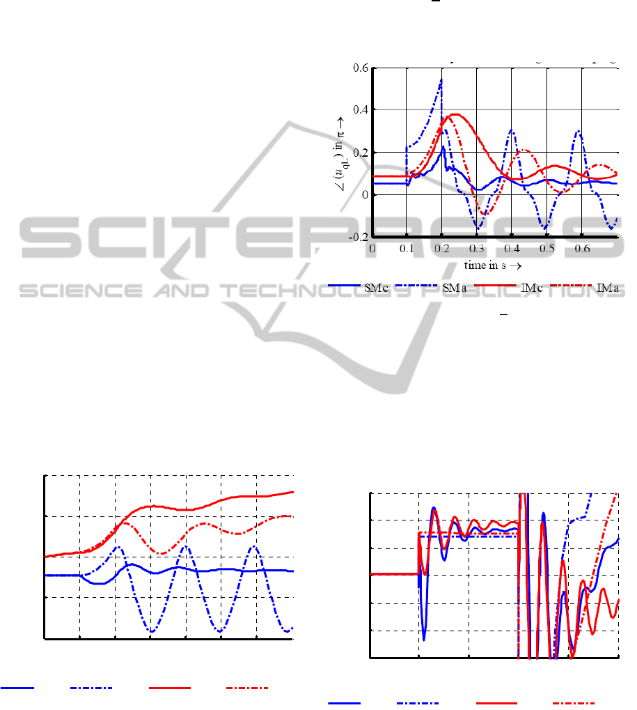
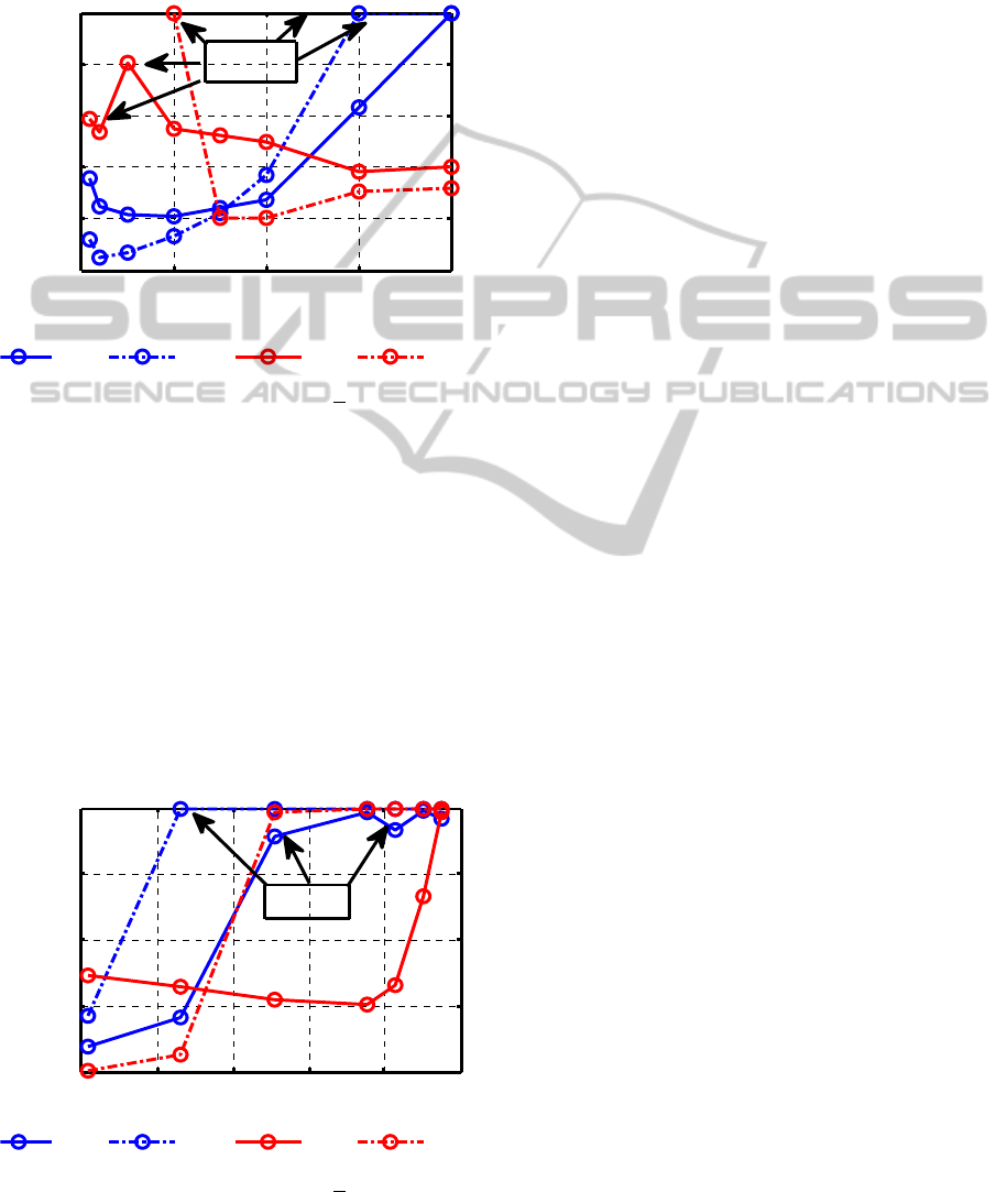
Figure 3: Angles of the voltage
qL
referred to the grid
angle around the fault in t = 0,1 s…0,2 s.
The deviance between the models during the
fault can be quite big for synchronous machines.
Also the oscillation after the fault has a weak
damping for the approximated models. As result
only machines based on the same model can be
compared quantitative. In the following sections this
will be done by comparing the maximal reached
angles referred to the angle of the overlaying grid.
Figure 4: Absorbed active power around the fault in
t = 0,1 s…0,2 s (zoom).
The deviance between the models is caused by
the approximations for stator currents and rotor flux
linkages. In the first part of the oscillation the
0 0.1 0.2 0.3 0.4 0.5 0.6
-1
-0.5
0
0.5
1
time in s
→
ϑ
LF
in
π
→
SM c SM a IM c IMa
0.05 0.1 0.15 0.2 0.25 0.
3
-4
-2
0
-4
-2
0
-4
time in s
→
active power in MW
→
SM c SM a IMc IMa
SIMULTECH2012-2ndInternationalConferenceonSimulationandModelingMethodologies,Technologiesand
Applications
372
consideration of the stator currents leads to a back
swing effect, which is caused by a significant
consumption of active power. The active power
consumption can reach significant levels due to the
displacement of the short circuit currents and the
resistances between the generation unit and the short
circuit point. This effect is very strong for the
synchronous machine. In the second part of the
oscillation the approximations for the rotor flux
linkages neglects the decay of active power. Please
note that the active power does not jump to zero due
to the resistive part of the grid impedance, which is
neglectable in high voltage grids.
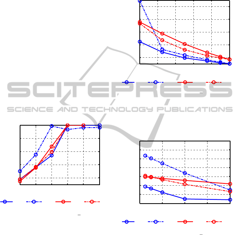
3.1.2 Different Durations
The duration of a short circuit in the 110-kV-grid
can reach some 100 milliseconds. The time is
determined by the reaction time of the protection
system and potential delays for selectivity reasons.
Both machines withstand short circuit durations
shorter than 200 milliseconds. Only the
approximated model of the synchronous machine
shows a wrong stability border.
Figure 5: Maximal angles of the voltage
qL
in relation to
the grid angle with different short circuit durations.
3.1.3 Different Residual Voltages
Depending on the real fault distance to the
transformer, the voltage drop can be smaller than
100 %. Small voltage drops can also be caused by
fast changes in the load flow.
All models show transient stability. In which the
approximated model of the synchronous machine
provided bigger values for the maximal voltage
angle amplitude, whereas the approximated
induction machine model provided lower values
than the corresponding complete models. In the
considered scenario the approximated model for the
synchronous machine works only properly with
residual voltages.
Figure 6: Maximal angles of the voltage
qL
in relation to
the grid angle with different residual voltages.
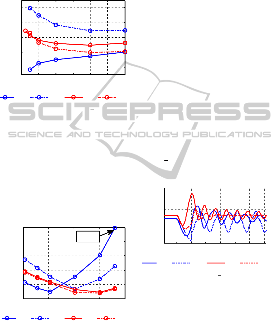
3.1.4 Different Line Lengths
The short circuit power at the point of common
coupling strongly depends on the line impedance
between the transformer T1 and the generation unit.
Figure 7: Maximal angles of the voltage
qL
in relation to
the grid angle with different line lengths.
With growing line length the generation units
gain transient stability. This is due to the resistive
part of the line impedance, which consumes a
significant amount of active power during the fault.
3.1.5 Different Rated Machine Powers
The rated power has an impact on the machine
parameters. This dependence is shown here for a
50 100 150 200 250 300
0.2
0.4
0.6
0.8
1
duration in ms
→
maximum angle of u
q
in
π
→
SM c SM a IMc IMa
0 20 40 60 80 10
0
0.1
0.2
0.3
0.4
0.5
residual voltage in %
→
maximum angle of u
q
in
π
→
SM c SM a IM c IMa
0 100 200 300 40
0
0.1
0.2
0.3
0.4
0.5
0.6
0.7
line length in %
→
maximum angle of u
q
in
π
→
SM c SM a IM c IMa
MachineModellingforTransientStabilityAnalysisinDistributionGrids-AComparisonofSynchronousandInduction
MachineModelsinMediumandLowVoltageGrids
373
range of possible values, without displaying the
array of implemented parameters.
Figure 8: Maximal angles of the voltage
qL
in relation to
the grid angle with different rated power of the machine.
With smaller rated power, the difference
between the complete and the approximated
synchronous machine model increase. With smaller
values the transient stability for synchronous
machines is enhanced and for induction machines
reduced.
3.1.6 Different Operation Points
In the previous scenarios the machines where always
initialized with rated power. In the classic approach
this is the worst case. The transient stability is
improved with lower machine utilization, because
the accelerating torque is higher.
Figure 9: Maximal angles of the voltage
qL
in relation to
the grid angle with different machine utilisation powers P.
In contrast to the high voltage grid the machine
in the distribution grid can be subject to a distinct
back swing effect. This leads to an optimal operation
point, which is effected by the impedance between
generation unit and fault. The approximated
induction machine model works very well with
different operation points. The approximated
synchronous machine model can pretend better
results than the exact model. So the instability of the
synchronous machine at 10 % could not be detected.
3.2 Low Voltage Scenario
Generation units in low voltage grids are easily
affected by a short circuit. To gain transient stability
in the basic scenario a residual voltage of 50 % was
assumed at the fault node. This can only be done,
keeping in mind the deviation of the approximated
model in the medium voltage scenario with residual
voltages.
3.2.1 Basic Scenario
The operation point depending gradient of the rotor
angles prevents the analyses of the transient stability
by the rotor angles development.
As alternative again the angles of the induced
voltages
qL
were checked for coherence. Also the
quantitative comparison will be done, by comparing
the maximal reached angles referred to the angle of
the overlaying grid.
Figure 10: Angles of the voltage
qL
referred to the grid
angle around the fault in t = 0,1 s…0,2 s.
The deviance between to models is caused by the
approximations for stator currents and rotor flux
linkages. All models show a back swing effect,
which is stronger for the approximated models. This
is due to the inaccurate modelling of the active
power exchange.
0 2 4 6 8 10 12
0.2
0.3
0.4
0.5
0.6
S
rG
in M VA
→
maximum angle of u
q
in
π
→
S
M
c
S
Ma IM
c
IMa
-2 -1.5 -1 -0.5 0
0
0.2
0.4
0.6
0.8
1
P in MW
→
maximum angle of u
q
in
π
→
SM c SM a IMc IMa
unstable
0.1 0.2 0.3 0.4 0.5 0.6 0.7
-0.4
-0.2
0
0.2
0.4
time in s
→
∠
(u
qL
) in
π
→
SM c SM a IM c IM a
SIMULTECH2012-2ndInternationalConferenceonSimulationandModelingMethodologies,Technologiesand
Applications
374
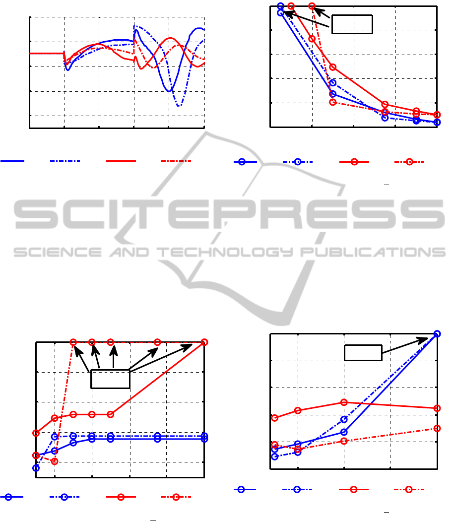
Figure 11: Absorbed active power around the fault in
t = 0,1 s…0,2 s (zoom).
3.2.2 Different Durations
The short circuit duration in distribution grids can
reach higher values than in the transmission grids.
This is due to simpler and slower protection systems.
The induction machine withstands a short circuit
durations smaller than 250 milliseconds. The
approximated model is not suitable for long short
circuit durations. The synchronous machine is able
to reach a new stable operation point. This is due to
the assumed residual voltage of 50 %.
Figure 12: Maximal angles of the voltage
qL
in relation to
the grid angle with different short circuit durations in s.
3.2.3 Different Residual Voltages
Depending on the real fault distance to the
transformer, the voltage drop can be smaller than
100 %. Small voltage drops can also be caused by
fast changes in the load flow.
Figure 13: Maximal angles of the voltage
qL
in relation to
the grid angle with different residual voltages.
In this scenario the models only show transient
stability for significant residual voltages at the 110-
kV node. The approximated models are faster to
show transient instability.
3.2.4 Different Line Lengths
The short circuit power at the point of common
coupling strongly depends on the line impedance
between the transformer T1 and the generation unit.
Figure 14: Maximal angles of the voltage
qL
in relation to
the grid angle with different line lengths in %.
With bigger line length the synchronous
generator loses transient stability. The approximated
models are able to reproduce the effects of different
short circuit impedances.
0.05 0.1 0.15 0.2 0.25 0.3
-6
-4
-2
0
2
x 10
5
time in s
→
active power in W
→
SM c SM a IMc IM a
0.1 0.2 0.3 0.4 0.5
0.2
0.4
0.6
0.8
1
duration in s
→
maximum angle of u
q
in
π
→
SM c SM a IMc IMa
unstable
20 40 60 80 100
0
0.2
0.4
0.6
0.8
1
residual voltage in %
→
maximum angle of u
q
in
π
→
SM c SM a IM c IM a
unstable
50 100 150 200
0
0.2
0.4
0.6
0.8
1
line length in %
→
maximum angle of u
q
in
π
→
SM c SM a IMc IM a
unstable
MachineModellingforTransientStabilityAnalysisinDistributionGrids-AComparisonofSynchronousandInduction
MachineModelsinMediumandLowVoltageGrids
375
3.2.5 Different Rated Machine Powers
The rated power has an impact on the machine
parameters. This dependence is shown here for a
range of possible values, without displaying the
array of implemented parameters.
Figure 15: Maximal angles of the voltage
qL
in relation to
the grid angle with different rated power of the machine.
With smaller rated power the difference between
the complete and the approximated synchronous
machine model increase. Similar to the medium
voltage scenario the transient stability of
synchronous machines is enhanced and for induction
machines reduced with smaller values for the rated
machine power.
3.2.6 Different Operation Points
In the other scenarios the machines where always
initialized with rated power. In contrast to the classic
model this is not the worst case.
Figure 16: Maximal angles of the voltage
qL
in relation to
the grid angle with different machine utilisation powers P.
The transient stability of synchronous and
induction machine is reduced with low active power
infeed, whereas the induction machine is affected at
relatively low values. The approximated models
show the transient instability afore.
4 CONCLUSIONS
The complete models of synchronous and induction
machines were compared with selected
approximated models of lower order. This is to
validate the approximations for the utilisation in
transient stability analysis in distribution grids.
A range of scenarios was analysed, to detect the
influence of different parameters in the model
accuracy. This was done comparing the maximal
angle amplitude of the modelled machine voltage
sources. Doing so, the temporally developing still
has to be taken in to account to detect all cases of
instability.
The results show that the approximated models
can be used to simulate stable oscillations, but they
lose their accuracy approaching the area of transient
instability. They can still be used to analyse positive
or negative effects on the transient stability.
The differences between the models are mostly
due to the modelling of the active power exchange
during fault, which is not jumping to zero as it does
in high voltage scenarios.
It has to be noted that the accuracy of the models
and also the transient stability strongly depend on
the rated and the actual power of the generation
units.
REFERENCES
Kundur, P., 2007. Power System Stability and Control,
Tata McGram-Hill. New York.
Oswald, B., 2009. Berechnung von Drehstromnetzen,
Vieweg+Teubner. Wiesbaden.
Hofmann, L., 2003. Effiziente Berechnung von
Ausgleichsvorgängen in ausgedehnten
Elektroenergiesystemen, Shaker Verlag. Aachen.
0 50 100 150 200
0
0.2
0.4
0.6
0.8
1
S
rG
in kVA
→
maximum angle of u
q
in
π
→
SM c SM a IMc IM a
unstable
-0.1 -0.08 -0.06 -0.04 -0.02 0
0.2
0.4
0.6
0.8
1
P in MW
→
maximum angle of u
q
in
π
→
SM c SM a IMc IMa
unstable
SIMULTECH2012-2ndInternationalConferenceonSimulationandModelingMethodologies,Technologiesand
Applications
376
