
Finding a Tradeoff between Compression and Loss in Motion
Compensated Video Coding
Thomas Guthier
1,2
, Adrian Sosic
1
, Volker Willert
1
and Julian Eggert
2
1
Control Theory and Robotics, TU Darmstadt, Landgraf-Georg Strasse, Darmstadt, Germany
2
Honda Research Institute Europe, Offenbach, Germany
Keywords:
Video Coding, Polynomial Motion Model, Quadtree Segmentation, Model Selection.
Abstract:
In video coding, affine motion models combined with a quadtree decomposition have often been suggested
as an extension to the mostly used translational models combined with a blockwise decomposition. What is
missing so far is a thorough analysis to judge the tradeoff between using more complex motion models or more
elaborate decomposition methods in terms of data compression and information loss. In this paper, we compare
different polynomial motion models with a quadtree decomposition concerning motion model complexity
and granularity of decomposition. We provide a statistical evaluation based on optical flow databases to
quantitatively find a tradeoff between bitrate and reconstruction error.
1 INTRODUCTION
One of the most important aspects in modern video
coding are motion compensation algorithms. Those
algorithms segment each image of the sequence and
describe the local motion of each segment. This mo-
tion information is then used to predict the recent im-
age given the image of the previous timestep. The
use of the temporal correlation in image sequences
can drastically reduce the bitrate. In lossy video cod-
ing, the quality of the compressed video will decrease
because of prediction errors of the motion compen-
sation. Therefore the quality requirements must be
balanced with bitrate requirements. While video cod-
ing standards like MPEG-4 or H.264 (Wiegand et al.,
2003) use only block-wise segmentation and purely
translational models to describe the local motion, a
lot of research focuses on more sophisticated motion
models and segmentation methods. An overview on
the recent development in video coding can be found
in (Sikora, 2005). For example (Zhang et al., 1997)
use a hierarchical segmentation including a quadtree
decomposition and affine models for motion com-
pensation. Their algorithm shows good results con-
cerning reconstruction quality and bitrate reduction
in highly structured scenes, but the bitrate exceeds
the coding standards in scences with little motion
due to the extra parameters needed for their com-
plex segmentation. (Karczewicz et al., 1997) use a
quadtree based segmentation along with polynomial
(a) (b)
Figure 1: On the left is an example image and on the right
the corresponding color coded flow field. The color value
codes the moving direction and the intensity the amplitude
of the motion. The lines show the quadtree segmentation.
motion models. The quadtree segmentation is easy
to implement and needs only one extra bit per seg-
ment compared to a regular block-wise segmentation
when using an efficient coding as described in (Sulli-
van and Baker, 1994). Their video coding algorithm
showed good results concerning both reconstruction
quality and compression, but is not realtime capa-
ble due to a complex coefficient selection algorithm
which is needed to reduce the number of bits en-
coding the polynomial motion models. (Lakshman
et al., 2010) focus on adaptivemotion model selection
to overcome the problem of the multiple parameters
needed to encode higher order polynomial models.
Although research is focusing on extensions of the
simple translational model and the block-wise decom-
position, little has been done to study the complex
interdependencies between the reconstruction quality,
81
Guthier T., Sosic A., Willert V. and Eggert J..
Finding a Tradeoff between Compression and Loss in Motion Compensated Video Coding.
DOI: 10.5220/0004057000810084
In Proceedings of the International Conference on Signal Processing and Multimedia Applications and Wireless Information Networks and Systems
(SIGMAP-2012), pages 81-84
ISBN: 978-989-8565-25-9
Copyright
c
2012 SCITEPRESS (Science and Technology Publications, Lda.)

the required number of bits, the segmentation algo-
rithm and the different model orders. The reconstruc-
tion quality depends on two elements: The model or-
der and the segmentation. A higher model order and
a finer segmentation both increase the reconstruction
quality, but then again increase the number of bits.
An open question is, whether an increased model or-
der can increase the reconstruction quality and addi-
tionally lead to a coarser segmentation and therefore
lower the overall required bitrate at the same time. Or
if on the other hand, a finer segmentation with simpler
motion models yields better results.
The topic of this paper is twofold. The first
achievement is a statistical analysis of the gain in re-
construction quality for increasing the order of poly-
nomial motion models. The second achievement is
the analysis whether it is a better strategy to spend
more bits on the segmentation and less on the model
complexity or vice versa. For the purpose of com-
parison two segmentation algorithms are used. One
simple block-wise segmentation familiar to the one
used in the MPEG4 standard and a quadtree de-
composition. Because this research focuses on mo-
tion compensation and not on an entire video cod-
ing algorithm, all experiments are directly done on
ground truth optical flow datasets and not on image
sequences.
2 ALGORITHM
In the following pixel positions in the images are de-
scribed by ~x = (x, y)
⊤
and flow fields are given by
the correspondingflow vectors~v(~x) = (v
x
(~x), v
y
(~x))
⊤
.
As a measurement of the reconstruction quality we
define the reconstruction error E
s
=
1
n
s
∑
~x
s
k~v(~x
s
) −
¯
~v(~p
s
,~x
s
)k
2
2
. k · k
2
is the Euclidean norm,
¯
~v(~x
s
) =
( ¯v
x
(~x
s
), ¯v
y
(~x
s
))
⊤
is the model of the optical flow and
n
s
= number of pixels per segment.
1
With s = num-
ber of segments, we get the normalized reconstruction
error E =
1
s
∑
s
E
s
.
2.1 Linear Parametric Models
The model order is N, the coefficients for v
x
(~x) are
~a = (a
0
,a
1
,...)
⊤
and for v
y
(~x) are
~
b = (b
0
,b
1
,...)
⊤
.
Polynomial models can be described by
1
We choose the reconstruction error instead of the more
popular PSNR to distinguish that we compare the flow
model to the ideal flow field and not the gray value pixel
values with the ones warped by the flow model.
¯v
x
(~x) =
N
∑
n=0
n
∑
i=0
a
n−i,i
x
n−i
y
i
,
¯v
y
(~x) =
N
∑
n=0
n
∑
i=0
b
n−i,i
x
n−i
y
i
.
Each segment has its own parameter vector ~p
s
=
(~a,
~
b). The number of parameters per model is
q
m
= 2
N
∑
n=0
n
∑
i=0
1 = (N + 1)(N + 2). (1)
The model of order N = 0 is the translational model
and has 2 parameters. The first order model is the
affine model with 6 parameters. The model param-
eters are estimated by minimizing the reconstruction
error.
2.2 Segmentation
There are two parameters controlling the segmenta-
tion process. The quality parameter ε and the max-
imum segmentation level l
max
. l is the segmentation
level. The algorithm for each segment is:
1. Calculate the model parameters p
s
.
2. Calculate the normalized reconstruction error E
s
.
3. If E
s
< ε ∨ l = l
max
⇒ stop. Else, continue
with step 4.
4. Divide the segment into four rectangluar seg-
ments. Increase the segmentation level counter
and continue for each new segment at step 1.
One result of this quadtree segmentation can be seen
in Fig. 1. For ε = 0 the algorithm has zero tolerance to
model errors and is likely to segment the entire flow
field into equally sized rectangluar blocks until l
max
is reached. This is comparable to the block-wise de-
composition proposed in the MPEG4 standard.
2.3 Dependency of Segmentation Level
and Model Order
Some dependencies have a theoretic nature and can be
directly derived from the formulars. In the following,
we show under which conditions a quadtree decom-
position leads to less parameters than a block-wise
decomposition and how increasing the model order
and the maximum segmentation level increases the bi-
trate. Let q be the number of parameters needed to
encode one timestep of a motion compensation algo-
rithm. When using block-wise decomposition (index
b
), no parameter is needed to encode the segmenta-
tion. For the quadtree decomposition (index
q
) one
SIGMAP2012-InternationalConferenceonSignalProcessingandMultimediaApplications
82

0 1 2 3 4 5 6
−3
−2
−1
0
1
2
3
Segmentation Level
Reconstruction Error (log)
0. Order
1. Order
2. Order
3. Order
4. Order
Figure 2: Mean value of the reconstruction error depend-
ing on the segmentation level for two optical flow datasets.
Each curve shows a different motion model.
extra parameter per segment is needed for the encod-
ing. We now compare the number of parameters q
q
versus q
b
with q
b
= s
b
·q
m
and q
q
= s
q
·(q
m
+ 1). The
inequality q
q
≤ q
b
leads to
s
q
s
b
≤
q
m
q
m
+1
. For low model
orders the number of quadtree segments s
q
has to be
smaller than the number of block segments s
b
to make
the quadtree decomposition more effective than the
block-wise segmentation. For higher model orders
the fraction
q
m
q
m
+1
converges towards one. Therefore
the influence of the extra bit for the quadtree decom-
position is decreasing. Next we analyze the increase
of q
b
due to an increase of N and l for a block-wise de-
composition. The number of segments s
b
(l) = 4
l
ex-
ponentially depends on the segmentation level l. With
eq. (1) we get q
b
(l, N) = (N + 1)(N + 2)4
l
and the
gain in q
b
:
∆q
b,l
= q
b
(l + 1,N) − q
b
(l, N) = 3(N + 1)(N + 2)4
l
,
∆q
b,N
= q
b
(l, N + 1) − q
b
(l, N) = 2(N + 2)4
l
,
∆q
b,l
∆q
b,N
=
3
2
(N + 1). (2)
Incrementing the segmentation level leads to extra
bits compared to incrementing the model order, de-
pending linearly on the model order.
3 SIMULATION RESULTS
3.1 Error Depending on Model Order
Segmentation is done with the block-wise decompo-
sition even though the quadtree decomposition shows
comparable results. The analysis is done on the en-
tire sequences of the CSAIL (Liu et al., 2008) and
Middelbury (Baker et al., 2007) database, which pro-
vide ground truth optical flow. The databases contain
0 0.01 0.02 0.03 0.04 0.05 0.06 0.07 0.08
4
5
6
7
8
9
10
Reconstruction Error
Number of Parameters (log)
Level 2
Level 3
Level 4
Level 5
Level 6
block−wise
Figure 3: Number of parameters depending on the recon-
struction error for different segmentation levels. The algo-
rithm using the affine motion model was applied to the car
sequence.
complex sequences with moving objects as well as
homogeneous regions and sequences with little mo-
tion. The curves in Fig. 2 show the mean values of all
sequences.
The curves are almost parallel throughout the dif-
ferent segmentation levels. Therefore the results are
independent of the segmentation quality. Increasing
the model order from translational to affine causes
the most segnificant increase in reconstruction qual-
ity. From eq. (2) we conclude that incrementing the
model order increases the bitrate less than increment-
ing the segmentation level. We now give an example
how this information can be applied to Fig. 2. We
start with the translational model (+) at the segmen-
tation level 3. The logarithmic reconstruction error is
≈ 1 and if we want to achieve ≈ 0 we can either in-
crease the segmentation level or the model order by
two. Because of eq. (2) latter is preferable.
3.2 Error and Bitrate Depending on the
Segmentation Level
In the following we use the affine model. Fig. 3
shows the results for different parameters l
max
and ε.
The algorithm was applied to the highly structured
car sequence of the CSAIL database that is shown in
Fig. 1. The simulations were performed for the other
sequences as well with comparable results. The seg-
mentation algorithm as described in Sec. 2 depends
on two parameters, the maximum segmentation level
l
max
and the quality parameter ε. If ε is set a low value
little errors are tolerated leading to a stronger segmen-
tation. Larger ε lead to higher reconstruction errors,
but less parameters. Each curve represents one l
max
and different ε, starting with ε = 0. The pareto front is
marked. For each bitrate and reconstruction error, the
FindingaTradeoffbetweenCompressionandLossinMotionCompensatedVideoCoding
83
0 0.01 0.02 0.03 0.04 0.05 0.06 0.07 0.08 0.09
5
6
7
8
9
10
11
12
Reconstruction Error
Number of Parameters (log)
0. r er
1. r er
2. r er
3. r er
4. r er
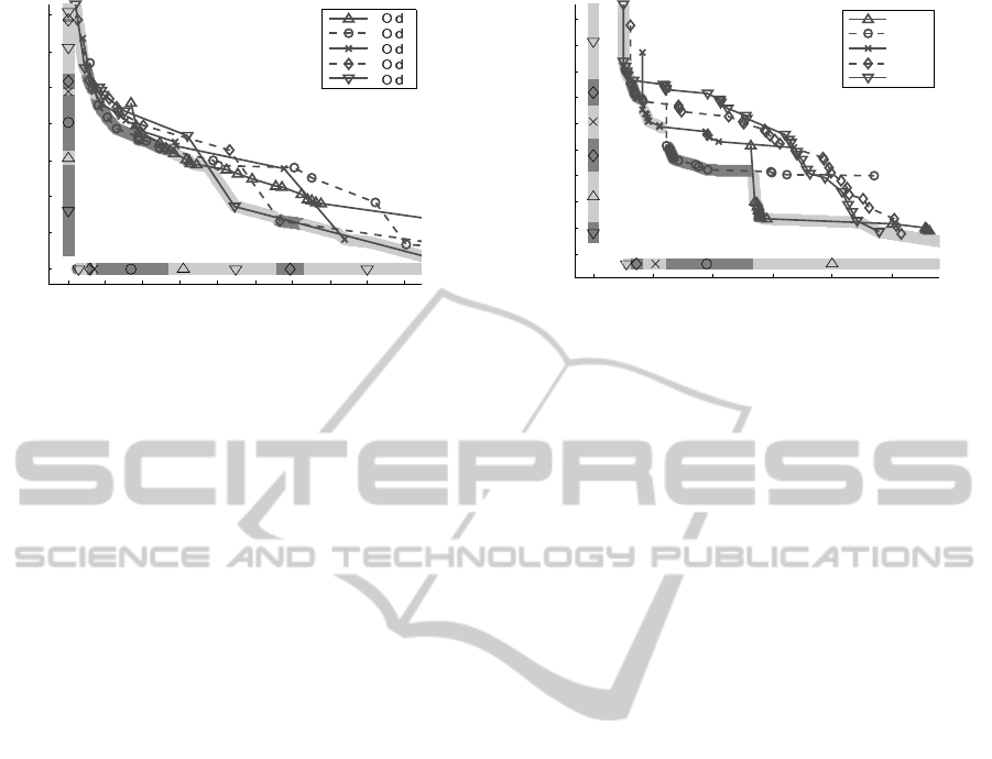
Figure 4: Number of parameters depending on the recon-
struction error for different motion models. The algorithm
segmented to the fifth level was applied to the car sequence.
ideal segmentation level is marked on the pareto front
that is additionally plotted next to the axis. The points
corresponding to a block-wise segmentation for each
l
max
are additionally marked in Fig. 3.
As discussed in Sec. 2 the block-wise segmenta-
tion yields the same reconstruction error as the corre-
sponding graph with ε = 0, but needs less parameters
to encode. From the points on the pareto front we
can conclude that the desired reconstruction quality
or bitrate can be achieved by adapting the segmenta-
tion level. There is no overall best segmentation level,
rather an ideal level for the different requirements.
3.3 Error and Bitrate Depending on the
Model Order
Next we fix the segmentation level l
max
= 5 and com-
pare the differentmodel orders and variousquality pa-
rameters ε. The results on the car sequence are plot-
ted in Fig. 4. Fig. 5 shows the same algorithm on
the hand sequence of the CSAIL database which has
on the one hand a lot of motion discontinuities and
on the other hand large homogeneous regions. Each
curve represents one polynomial motion model and
different ε, starting with ε = 0. Like in Fig. 3 the
pareto front is marked and additionally plotted with
the corresponding model next to the axis. For both
sequences there are regions on the pareto front where
one model gives the best tradeoff between bitrate and
reconstruction quality. Small reconstruction errors re-
fer to larger models.
4 CONCLUSIONS
We provide a qualitative and quantitative analysis for
motion compensation in video coding to find the best
0 0.5 1 1.5 2 2.5
7.5
8
8.5
9
9.5
10
10.5
11
11.5
12
Reconstruction Error
Number of Parameters (log)
0.Order
1.Order
2.Order
3.Order
4.Order
Figure 5: Number of parameters depending on the recon-
struction error for different models. The algorithm seg-
mented to the fifth level was applied to the hand sequence.
tradeoff given compression and loss constraints. It is
possible to judge which segmentation granularity and
motion model complexity best fulfills the coding re-
quirements. The results stress the need for coding al-
gorithms that are adaptive in both the segmentation
level and motion model order.
REFERENCES
Baker, S., Scharstein, D., Lewis, J. P., Roth, S., Black, M. J.,
and Szeliski, R. (2007). A database and evaluation
methodology for optical flow. In Proc. IEEE Conf.
ICCV.
Karczewicz, M., Nieweglowski, J., and Haavisto, P. (1997).
Video coding using motion compensation with poly-
nomial motion vector fields. Signal Processing: Im-
age Communication, 10(1-3):63 – 91.
Lakshman, H., Schwarz, H., and Wiegand, T. (2010). Video
coding with cubic spline interpolation and adaptive
motion model selection. In SPCOM, Conf.
Liu, C., Freeman, W. T., Adelson, E. H., and Weiss, Y.
(2008). Human-assisted motion annotation. In Proc.
IEEE Conf. CVPR, pages 1–8.
Sikora, T. (2005). Trends and perspectives in image and
video coding. IEEE J.PROC., 93(1):6–17.
Sullivan, G. J. and Baker, R. L. (1994). Efficient quadtree
coding of images and video. IEEE J.PROC., 3.
Wiegand, T., Sullivan, G., Bjontegaard, G., and Luthra, A.
(2003). Overview of the h.264/avc video coding stan-
dard. IEEE Transactions on CSVT, 13(7):560 –576.
Zhang, K., Bober, M., and Kittler, J. (1997). Image se-
quence coding using multiple-level segmentation and
affine motion estimation. Selected Areas in Commu-
nications, IEEE Journal on, 15(9):1704 –1713.
SIGMAP2012-InternationalConferenceonSignalProcessingandMultimediaApplications
84
