
SysML Parametric Models for Complex System Performance Analysis
A Case Study
Nga Nguyen and Hubert Kadima
Laris, EISTI, Avenue du Parc, 95011 Cergy, France
Keywords: Model-based System Engineering, SysML Parametric Diagram, Performance Analysis, Cruise Control.
Abstract: Parametric analysis is an essential tool in optimizing the performance of any system; it is, in particular, used
to fine-tune key parameters in a system design process. In this paper, using a vehicle cruise control system
as a non-trivial case study, we introduce a new approach for the performance parametric analysis of
complex systems using SysML models and a parametric constraint solver. System requirements are taken
into account to verify automatically whether the design solutions satisfy these requirements. This suggests
that in order to reduce time and resources, it is possible to perform initial performance analysis in a
modeling tool, just after the system functional and architectural analyses. Of course, once an approximate
operating point has been determined using this approach, experiments in specialized simulation tools can be
used to confirm and further refine the parameters of a system.
1 INTRODUCTION
SysML (SysML, 2010) is a visual modeling
language used to support the specification, analysis,
design, verification and validation of any engineered
system. Taking advantage of SysML concepts such
as requirements, blocks, flow ports, parametric
diagrams and allocations, it is easy to model
architectural and operational aspects of complex
systems at various levels of abstraction.
In this paper, we perform a sensitivity analysis,
which explores a parameter space, to find ideal
operational parameters allowing the validation of
alternative operational scenarios and system
configurations. The impact of constraints on system
properties and behaviours is analyzed in order to
optimize global system performance. We use
conjointly SysML parametric diagrams and a solver
in support of analyzing system alternatives
performances with respect to stakeholder
requirements, derived system requirements and
measures of effectiveness.
To illustrate our approach, we use a particular
case study: a Cruise Control Engine system. Since
many design parameters influence the operation of
such a system, it is difficult to quantify their impact
on the interactions within the system, and thus its
performance. The purpose of this study is thus to
investigate the consequences of varying some of
these operating parameters on the performance of
the system and to report the results using more
quantitative measures. The outcomes will be used to
improve the understanding of the system operation
and to optimize its performance by changing some
operating parameters or improving components. Due
to the large parameter space, and the complex,
highly coupled hybrid nature of the different internal
components of automatic systems, analysis is
complicated and sometime more specialized
simulation tools are necessary. The limits of our
approach are also discussed.
The structure of the paper is the following. In
Section 2, we describe briefly the functionalities of a
cruise control engine, the related SysML
requirement diagram and the dynamic model used in
our case study. Section 3 presents the parametric
analysis using the IBM Rhapsody SysML IDE,
SysML parametric models and IBM add-on
parametric constraint evaluator. Some preliminary
parametric analysis of dynamic constraints in trade-
off design activities and results of the case study are
discussed in Section 4. Conclusions are outlined in
Section 5.
2 CRUISE CONTROL SYSTEM
2.1 Functionalities
Cruise control is a system that automatically controls
321
Nguyen N. and Kadima H..
SysML Parametric Models for Complex System Performance Analysis - A Case Study.
DOI: 10.5220/0004058603210327
In Proceedings of the 2nd International Conference on Simulation and Modeling Methodologies, Technologies and Applications (SIMULTECH-2012),
pages 321-327
ISBN: 978-989-8565-20-4
Copyright
c
2012 SCITEPRESS (Science and Technology Publications, Lda.)
the speed of a vehicle by maintaining a constant
speed set by the driver. The implementation of a
cruise control system may vary but respects in
general the following principles. First, the cruise
control system may need to be turned on before use:
it passes from the disengaged state to the engaged
state. While engaged, cruise control becomes
activated when the driver sets the desired speed. A
driver instruction, such as braking or throttle pedal
depression, will put the cruise control on suspended
mode. Of course, we can easily go back to the
configuration before the suspension by using the
resume function supported by almost all systems.
Beside these operations, one can always increment
or decrement the desired speed when the system is
activated.
2.2 Requirements Model
Requirements analysis is the first step in the system
design process, where stakeholder requirements are
translated into system requirements that define what
the system must do and how well it must perform.
The result is a requirement diagram in which the
requirements are classified hierarchically. Complex
specifications are decomposed and categorized into
simpler ones, leading to a better interpretation that
will help with system verification and validation.
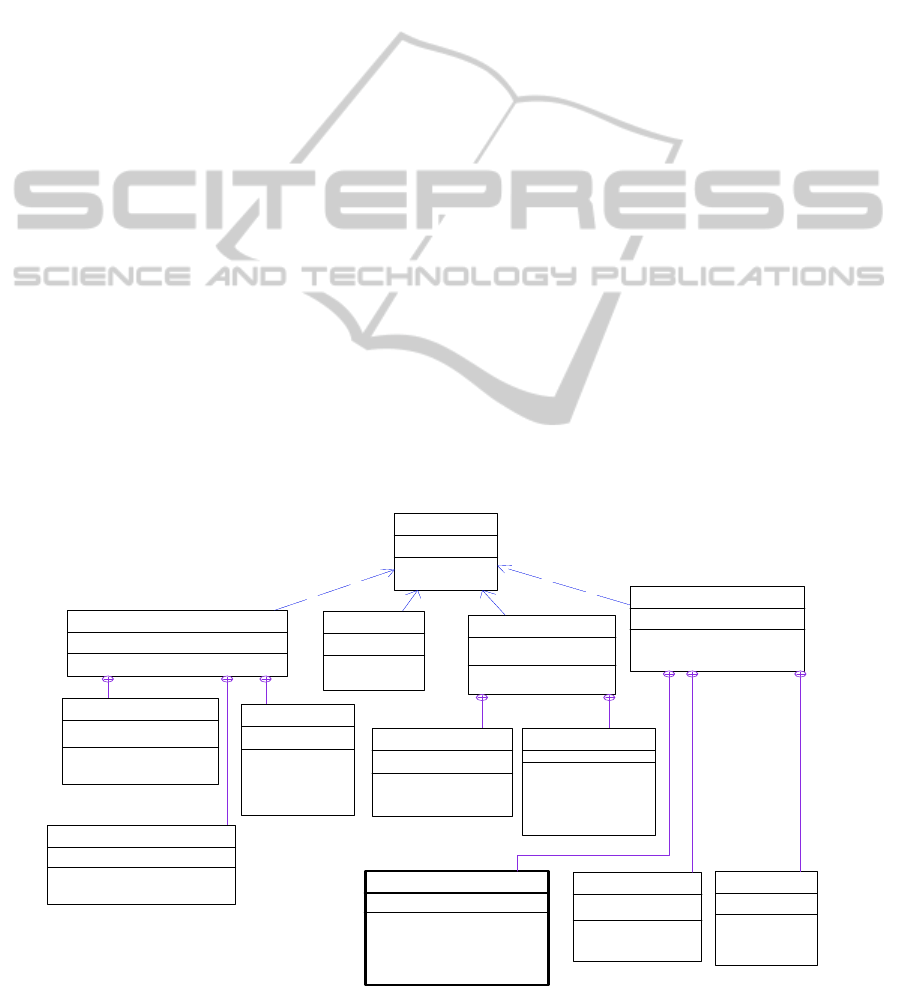
Figure 1 shows the requirement diagram for our
cruise control system. In the performance
requirement category, you can see some design
constraints for cruise control systems taken from
Control Tutorials for Matlab (Michigan, 1997), with
some of our own modifications. For example, when
the motor yields a 1500 Newton force, the car must
reach a maximum velocity of 30 m/s and be able to
accelerate up to that speed in less than 5 seconds.
Beside this, a 10% overshoot on the car speed and a
2% steady-state error are acceptable for the cruise
control system. The above criteria can be used later
to verify if the design solutions respect these
requirements. To complete the requirement analysis
phase, a model for system use cases must be built to
establish traceability links between requirements and
use cases provided, in order to ensure the coverage
of functional and performance requirements by the
use cases. These issues fall outside the scope of this
paper.
2.3 Dynamic Model
Almost all cruise control systems follow the closed-
loop control system principle. A sensor monitors the
car speed and feeds data to a controller that adjusts
the control as needed to maintain the reference
speed. When the car goes uphill or downhill, the
difference in speed is measured, and the throttle
position changed to increase or decrease engine
power, speeding or slowing respectively the vehicle.
Feedback from measuring the car velocity allows the
controller to dynamically compensate for changes to
the car speed.
Figure 1: Requirement Diagram of a Cruise Control.
Cruis e C ontrol
«R equireme nt»
ID = 001
Maintain a
constant
sp eed .
«derive»
Functional Managem ent
«R equire ment»
ID = 0 02
Ma nage the vario us operational
modes
«derive»
«derive»
Operational Safety
«R equire ment»
ID = 004
The system must be
sa fe and
comfortable
«derive»
Us er Interface
«Require me nt»
ID = 0 03
A generic
us er
interface is
id
«derive»«derive»
Enga ge-Disengage
«R equire ment»
ID = 007
The s ystem can be in the
engaged state or
disengaged state.
Spee d Settings
«R equire me nt»
ID = 0 08
The s peed
va lu e c a n be
chang ed by
incrementing
or
decrementing
b
y
a fi xed s te
p
.
Suspend-Resum e
«R equire ment»
ID = 0 06
The s ystem c an be
suspended or
resumed after
suspension
Displ ay
«R equireme nt»
ID = 0 09
Th e s yste m h a ve to
display the
information at any
tim e.
Errors
«R equireme nt»
ID = 010
Al l t h e e rr or s
encountered by the
system have to be
logged, except in
the di sen gag ed
mode.
«derive»
Performance Constrain ts
«R equireme nt»
ID = 005
The system must satisfy
so me behavioral
constraints
«derive»
Spee d and Time Lim it
«R equire ment»
ID = 0 12
When the en gine
generates about 1500
Newton force; the ca r m ust
reach its ma ximum speed
wh ich is 30 m s/s in les s
than 5 seconds
Exceedin g Speed
«R equireme nt»
ID = 0 123
Exceedin g 10 % of
desired s peed is
acceptable
Stabil ity Error
«R equire ment»
ID = 0 11
A stability
error of 2% is
acceptable
SIMULTECH2012-2ndInternationalConferenceonSimulationandModelingMethodologies,Technologiesand
Applications
322

PID (proportional - integral - derivative)
controller is widely used in industrial control system
theory. The typical form of the PID algorithm is the
following:
(
)
=
(
)
+
(
)
+
(
)
where k
p
, k
i
and k
d
are tuning parameters that have to
be adjusted to optimum values to achieve the desired
response while maintaining the stability of the
system. The control signal u computed by the
controller is used to rectify the throttle position and
thus the torque delivered by the engine, generating a
force that accelerates the vehicle.
To illustrate our case study, we used the dynamic
model of a cruise control system found in Astrom
and Murray's book (Astrom and Murray, 2010).
Their proportional - integral (PI) controller has the
form:
(
)
=
(
)
+
(
)
=
−
where v
r
is the desired speed, v the current speed
and u the signal control. The torque T, controlled by
the throttle position, delivered by the engine and
transmitted through the gears and the wheels,
depends also on engine speed ω:
(
)
=
1−
−1
where the maximum torque T
m
is obtained at engine
speed ω
m
, and typical values are given for T
m
, ω
m
and β. The angular velocity is related to the speed
through the expression:
=
And the driving force generated by the torque T is
written as:
=
()
Typical values of α
n
(n is the gear ratio) for gears
1 through 5 are 40, 23, 16, 12 and 10. The car's
motion is given by the following equation:
=−
where m is the mass, F
d
the disturbance force which
has three major components : gravity force (F
g
),
rolling friction force (F
r
) and aerodynamic drag
force (F
a
). Different parameters such as the slope of
the road, total mass of the car, gravitational constant,
density of air, frontal area of the car as well as
coefficients of various forces are taken into account
in the model.
3 PARAMETRIC ANALYSIS
In this section, we provide information regarding the
main components of our tools environment. Good
tool integration is paramount here, since round-trip
interoperability between SysML parametric models
and an integrated solver is a key requirement of our
approach.
3.1 SysML Parametric Models
SysML provides mechanisms and constructs
necessary to successfully describe all the structural
and behavioural specifications and constraints of a
model of a system. In the design phase, it is
essential to annotate these models with qualitative
and quantitative requirements, known as non-
functional properties, aiming at verifying and
validating the temporal behaviour, power estimation
and other various constraints.
Block diagrams are the natural approach used by
SysML for expressing system-level models,
providing a standardized form of representation for
both the structure of a system and the equations that
characterize its dynamic and its functional and
behavioural constraints. Blocks are extended into
constraint blocks that can be used in parametric
diagrams, which enable users to model equations in
terms of constraints in SysML, establishing a
network of relations among the properties of a
system (Peak, et al., 2007). These mathematical
expressions can represent the physical properties of
a system (e.g., relevant physics laws) or non-
functional properties (e.g., cost, risk, performance,
reliability, etc).
Simulation and system parametric analysis then
can be realized to check that a system definition
meets a certain system requirement, which can be
modelled explicitly using the SysML “verify”
dependency stereotype. Furthermore, some non-
functional requirements can be written as constraints
so they can be automatically verified by an
integrated solver. Instead of using specific
simulation tools such as Simulink or Modelica, we
decided to exploit a lightweight solver already
integrated in a SysML supported toolset to carry out
parametric analyses.
3.2 IBM Rhapsody Toolset
IBM Rational Rhapsody(Hoffmann, 2010) is a
collaborative, model-based systems engineering
development platform providing simulation for early
requirement, architecture and behavioural validation.
SysMLParametricModelsforComplexSystemPerformanceAnalysis-ACaseStudy
323
We decided to use it in our research because it
provides tools to dynamically analyze and execute
SysML parametric diagrams to assist in trade study
analysis. The integrated Parametric Constraint
Evaluator is a Rhapsody add-on that allows the
evaluation of parametric diagrams via a Computer
Algebra System (CAS) that solves the corresponding
mathematical expressions. Matlab Toolbox and
Maxima are two CAS supported by IBM Rhapsody;
given its ready availability, we chose the open-
source Maxima for this work. Maxima manipulates
symbolic and numerical expressions, and includes
many operations such as differentiation, integration,
Taylor series expansion, Laplace transform, ordinary
differential equation solving, systems of linear
equations manipulation, etc. It yields high precision
numeric results, using exact fractions and variable
precision floating point numbers. Thanks to
Maxima, PCE is able to compute the values that
satisfy mathematical constraints or to solve
constraints to minimize or maximize a value of an
attribute for linear algebraic equations. Besides this,
it can also produce graphs showing how values
behave over time or over a range of values of other
parameters. These possibilities allow a system
engineer to analyze the behaviours of the system, to
validate the constraints and to perform trade studies.
However, some solver limitations that are discussed
later led us to an interesting debate about the choice
of lightweight simulation tools such as parametric
diagrams with respect to dedicated tools such as
Simulink or Modelica.
4 SENSIBILITY ANALYSIS
Instead of using specialized simulation tools, we
have tried to use the SysML parametric diagram
coupled with a solver to carry out 2 different
simulations: an open loop cruise control as in
(Michigan, 1997) and a closed loop with the
dynamic model in Section 2.3. Throughout our
experiments, the limits of the solver integrated in
Rhapsody were encountered and are discussed here.
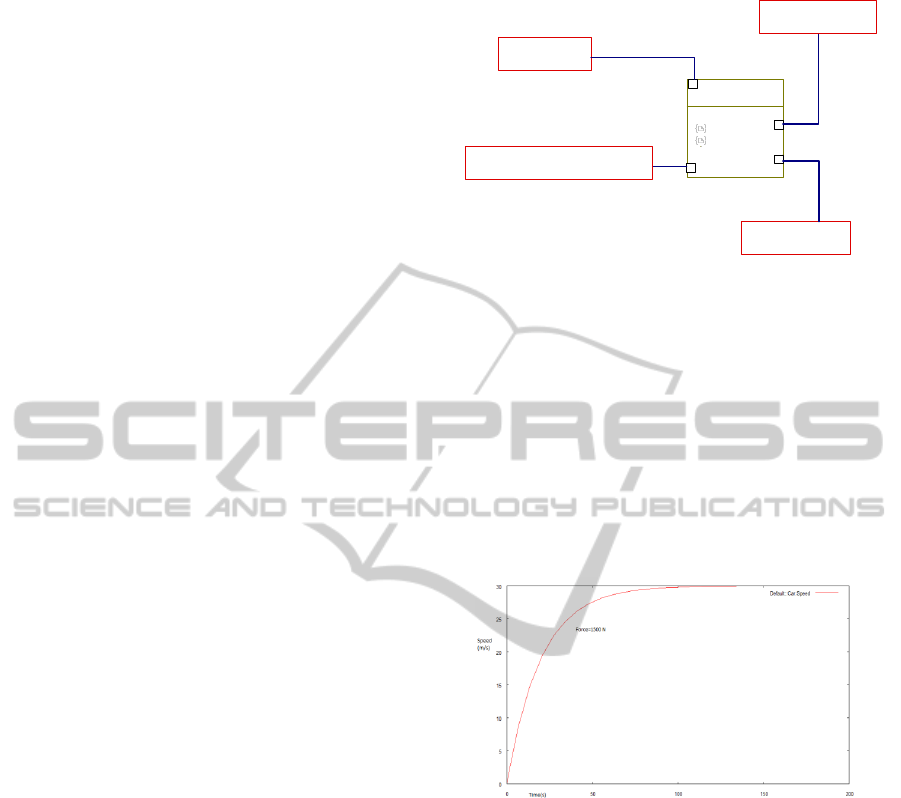
4.1 Open Loop Cruise Control
For an open loop experiment with linear differential
equations, our solver with Maxima succeeded at
producing desired results as with Matlab from the
parametric diagram in Figure 2.
Figure 2: Parametric Diagram of an Open Loop Cruise
Control.
We used here the same physical setup and system
equations as in (Michigan, 1997): friction opposing
the motion of the car is proportional to the car speed.
With an initial condition, a graph is generated from
the constraint view referencing the corresponding
parametric diagram, which is shown in Figure 3.
From the plot, we see that the car needs more than
100 seconds to reach the steady-state speed of
30m/s, which does not satisfy the performance
requirement about rise time (less than 5 seconds).
Figure 3: Speed vs. Time in Open Loop Cruise Control
(generated by PCE/Maxima).
4.2 Closed Loop with Dynamic Model
Our second implementation is the dynamic model of
the cruise control system described in Section 2.3.
The corresponding SysML parametric diagram is
provided in Figure 4. Each parametric constraint
represents an equation dealing with the comparator,
the controller, the torque related to the throttle
position, the generated force, the car motion and the
different disturbance forces. Constants are given in
the value properties. Almost all physical units are
available in the Systems Engineering (SE) profile of
Rhapsody.
Some simplifications have been made due to
software limitations: not all the possibilities of
Maxima are fully implemented. As PCE does not
Car Motion
1 «Cons traint P roperty»
Co ns t r a i nts
m*der(v)+b*v=f
v( 0) =0
f:Real
b:Real
m:K ilo gr am
v: Mete r Per Se con d
Mass:Kilogram=1000
«Attribu t e»
Speed:MeterPerSecond
«Attribu t e»
For ce: Newton=1500
«Attribute»
Friction Coef:NewtonSecondperMeter=50
«Attribu t e»
SIMULTECH2012-2ndInternationalConferenceonSimulationandModelingMethodologies,Technologiesand
Applications
324
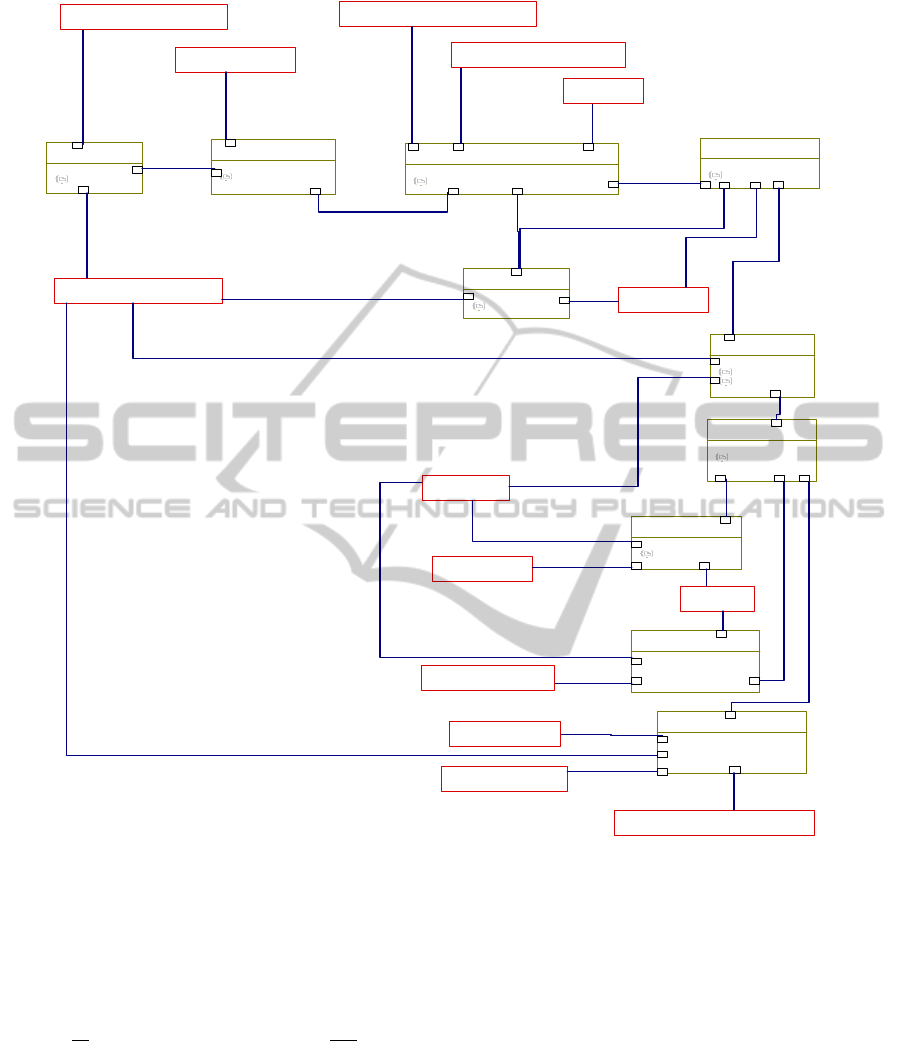
Figure 4: Parametric Diagram of the Dynamic Model.
support the integral operation or the Laplace
transform, we had to give up the integral part of the
controller; only proportional gain is taken into
account in the controller. That gives us the following
nonlinear differential equation for the system:
=
(
−
)
1−
−
1
–
−0.5
−sin(1)
where the last three terms represent respectively the
three disturbance forces : rolling friction,
aerodynamic drag and gravity force. Every variable
of the equation, except speed (v) and time (t), is
either constant or of known values.
A constraint view referencing the above
parametric diagram can be generated, as shown in
Figure 5. Normally, through the fixing of some
values in the spreadsheet, such as the value for the
proportional gain, the road slope, the car mass, the
desired speed…, we can ask Rhapsody to evaluate
the system in order to detect inconsistent constraints
or to display graphs that show interesting
relationships, for instance between time and speed.
Unfortunately, since Maxima only gives us the
exact analytical solution for the nonlinear
differential equation (1), which is not exploitable,
PCE cannot be used here. So, we decided to fall
back to using Scilab, an open-source solver using
numerical solutions, which allowed us to plot graphs
that represent the relationship between speed and
time from Equation (1), when varying some system
Engine S pee d
1 «C onstr aintProperty»
Constr aints
w=alpha*v
alpha
w:RadianPerSecond
v:Real
Current Speed:MeterPerSecond
«Attri bute »
Torque
1 «C onst rai ntPr oper ty»
Constrai nts
T=u*Tm*(1-B*(w/wm-1)*(w/wm-1))
u:Real
T:NewtonMete
r
B:Real
w:RadianPerSecond
wm:RadianPerSecond
Tm:NewtonMeter
MaxTorque:NewtonMeter=190
«Attri bute »
Max Engine Speed:RadianPerSecond=42
0
«Attr ibute»
Beta:Real=0.4
«Attr ibute»
Gravity Force
1 «C onst rai ntPr oper ty»
Const r ai nt s
Fg=m*g*sin(t...
Fg:Newton
teta:Radian
g:MeterP
m:Kilogram
Grav ity :Meter
P
«At tr ibu te »
Mass:Kilogr am
«Attr ibute»
Road Slope:Radian
«Attr ibute»
Rolling Friction Force
1 «ConstraintProperty»
Constraints
Fr=m*g*C1
Fr:Newton
m:Kilogram
g:MeterPerSe
C1:R e a l
Rolling Friction:Real=0. 01
«At tr ibu te »
Aerodynamic D rag Force
1 «C o nst rai ntProperty»
Constraints
Fa=0.5*Rho*Cd*A*v*v
Fa:Newton
v:MeterPerSecond
Rho:KilogramPerCubicMete
r
Cd:R e a l
A:MeterSquare
Car F rontal Area:Mete
r
«Attr ibute»
Aero drag Coef :Real=0.3
2
«Attr ibute»
Air Density :KilogramPerCubicMeter=1.3
«Attri bute »
Distu rb ance Fo rce
1 «ConstraintProperty»
Con s t r ai nt s
Fd=Fr+Fg+Fa
Fd:Newton
Fa:Newton
Fr:Newton
Fg:Newton
Car M oti on
1 «ConstraintProperty»
Constr aints
m *d er(v)=F-Fd
v(0)=0
Fd:Newton
F:Newton
v:MeterPerSecond
m:Kilogram
Force
1 «C onst rai ntPr oper ty»
Cons t r ai nt s
F=alpha*T
alpha
F:Newto n
T:NewtonMete
r
w:RadianPerSecond
Comp
1 «Co nst rai ntPr oper ty
»
Constraints
error=v r-v
error:Re a l
v:MeterPerSecond
vr:MeterPerSecond
Des ired Speed:MeterPerSecond
«Attr ibute»
Controller
1 «C ons tr aint Pr oper ty»
Constr aints
u=Kp* e rro r
u:Real
Kp:Real
error:Real
Proportional Gain:Real
«At tr ibu te »
Gear Rat io:int=1
0
«At tr ibu te »
SysMLParametricModelsforComplexSystemPerformanceAnalysis-ACaseStudy
325
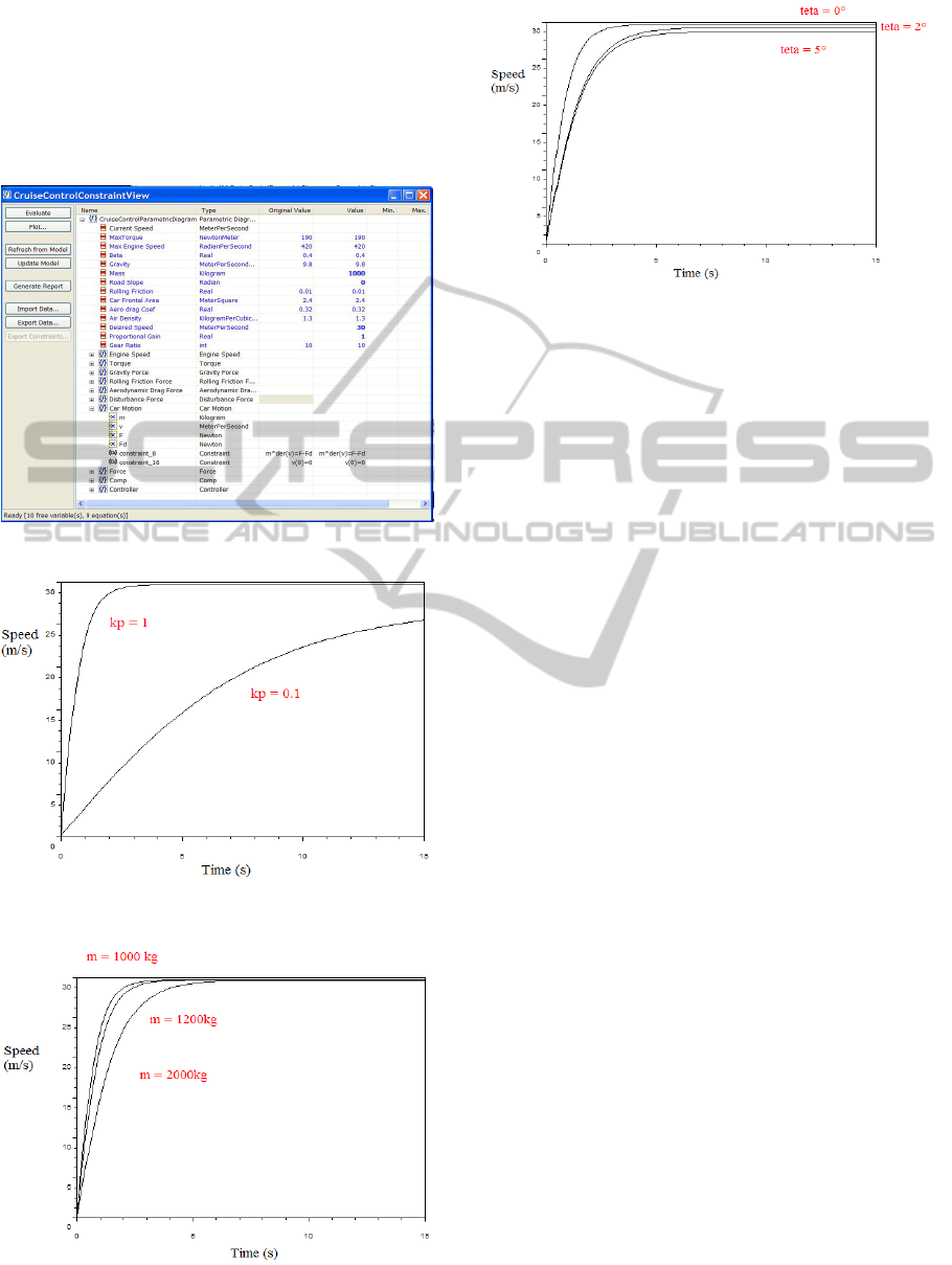
parameters. Some experimental results are given in
Figure 6, 7 and 8.
In Figure 6, we see that with k
p
= 1, the car
almost reaches the desired speed which is 30 m/s in
less than 5 seconds, so the performance
requirements about steady-state error and rise time
are verified.
Figure 5: Constraint View of the Dynamic Model.
Figure 6: Speed vs. Time with Different Proportional
Gains (generated by Scilab).
Figure 7: Speed vs. Time with Different Masses
(generated by Scilab).
Figure 8: Speed vs. Time with Different Road Slopes
(generated by Scilab).
With k
p
= 0.1, the system also arrives at the desired
target speed, but with a much longer rise time. In
Figure 7, by varying the total mass of the car and
keeping the value 1 for k
p
, we get different traces in
which only the trace for m = 1000 kg verifies the
condition of rise time less than 5 seconds. For the
other values of mass, further parameters must be
adjusted to achieve satisfying results. In Figure 8, by
varying the road slope while keeping the same value
for k
p
and m (1 and 1000kg respectively), we get
different outcomes. Since the vehicle has to provide
much more effort to go uphill (θ = 2° and 5°), with
the same value of k
p
, it cannot reach the desired
speed of 30 m/s.
The above results show that more experiments
must be run in order to find out optimum values for
the system parameters. All possible combinations of
the different value ranges for mass, road slope,
desired speed, etc must be taken into account. And,
of course, the integral and derivative gains are
necessary if we want to have more precision with
our cruise control system.
5 CONCLUSIONS
Due to the large parameter space and the highly
coupled hybrid nature of the different internal
components of automatic systems, their analysis is
usually complex and time consuming. In the case of
performance analysis, rather than performing
complete parametric analyses of complex systems in
the field, our paper suggests that initial parametric
performance analyses can be performed, in the lab,
using SysML parametric diagrams as main tool,
while at the same time leveraging conventional
modeling and simulation tools including
spreadsheets, math solvers, finite element analysis,
discrete event solvers and optimization tools. This
SIMULTECH2012-2ndInternationalConferenceonSimulationandModelingMethodologies,Technologiesand
Applications
326

approach allows for greater repeatability and
requires less time and resources. Of course, once an
approximate operating point has been determined
using this approach, field experiments with more
specialized tools (Simulink, OpenModelica, ...) can
be used to confirm and further refine the parameters
of a system.
Some works have been done by an OMG group
for the integration of SysML and Modelica to profit
the strength of two complementary modeling
languages: the descriptive power from SysML and
the analytic and computational power from
Modelica (Johnson and Jobe and Paredis and
Burkhart, 2007), (Paredis, et al., 2010). In fact,
Modelica is well suited for representing differential
algebraic equations to model the flow of energy,
materials, signals ... in complex system.
Transformation specification has been proposed to
provide a bi-directional mapping between the two
languages. However, the requirement models of
SysML are not considered in this mapping. In our
approach, we can integrate requirement information
directly into parametric diagrams to validate the
design. By rewriting requirement constraints in a
formal language such as OCL or a temporal logic
language, we can put them in the parametric
diagrams and then formal methods can be used to
verify if there are errors in system design.
The preliminary results presented in this paper
are quite encouraging. With a lightweight system,
we achieved results similar to those provided using
specialized tools and the perspective to be able to
combine directly in the same tool structural and
behavioural specifications with requirement
constraints to validate the design process is
promising.
Nevertheless, this solution presents some
limitations: although parametric diagrams are non-
causal, they do not separate effort and flow
variables, which is a fundamental issue when
modeling physical systems. For example, Modelica
(using flow) and VHDL-AMS (using
across/through) contain such constructs. Beside this,
although the Rhapsody tool is well suited for
implementing the first steps of complex system
development process, i.e., requirement analysis,
system functional analysis and design synthesis, the
architecture mismatch in its Parametric Constraint
Evaluator integrated with Maxima should be
corrected to represent more complicated
mathematical relations. For instance, a solver
providing numerical solutions for nonlinear
differential equations and supporting Laplace or Z
transforms (Wescott, 2012) would be highly
appreciated.
The next step of our work is to make a complete
survey of different SysML parametric solving tools
such as ParaSolver for Artisan Studio, ParaMagic
for MagicDraw, etc. in order to compare how far
these tools are able to support complex system
models. Actually, the tutorial examples given by
these tools are rather not very complicated.
REFERENCES
University of Michigan, http://www.engin.umich.edu/
group/ctm/examples/cruise/cc.html, 1997.
OMG Systems Modeling Language, Version 1.2, Juin
2010.
H. Hoffmann. Systems Engineering Best Practices with
the Rational Workbench for Systems and Software
Engineering, Deskbook Release 3.1.1. Model-Based
Systems Engineering with Rational Rhapsody and
Rational Harmony for Systems Engineering, 2010.
T. Johnson, J. Jobe, C. Paredis, and R. Burkhart. Modeling
Continuous System Dynamics in SysML. In IMECE,
2007.
C. J. J Paredis, Y. Bernard, R. M. Burkhart, H. P.
de Koning, S. Friedenthal, P. Fritzson, N.F. Rouquette,
and W. Schamai. An Overview of the SysML-
Modelica Transformation Specification. In INCOSE
International Symposium, 2010.
R. S. Peak, R. M. Burkhart, S.A. Friedenthal, M.W.
Wilson, M. Bajaj, and I. Kim. Simulation-Based
Design using SysML–Part 1: A parametric primer. In
INCOSE International Symposium, 2007.
R. S. Peak, R. M. Burkhart, S. A. Friedenthal, M.W.
Wilson, M. Bajaj, and I. Kim. Simulation-Based
Design using SysML–Part 2: Celebrating diversity by
example. In INCOSE International Symposium, 2007.
K. J. Åström and R. M. Murray. Feedback Systems: An
Introduction for Scientists and Engineers. Princeton
University Press, 2010.
T. Wescott. Z Transforms for the Embedded System
Engineer. Wescott Design Services.
SysMLParametricModelsforComplexSystemPerformanceAnalysis-ACaseStudy
327
