The Application of Evolutionary Algorithm for the Linear Dynamic

System Modelling

Ivan Ryzhikov and Eugene Semenkin

Institute of Computer Sciences and Telecommunication, Siberian State Aerospace University,

Krasnoyarskiy Rabochiy ave., 31, Krasnoyarsk, 660014, Russia

Keywords: Linear Dynamic System, Linear Differential Equation, Evolutionary Strategies, Parameters Identification

Problem, Structure Identification.

Abstract: The approach to dynamic system modelling in the linear differential equations form is presented. The given

approach fits the identification problems with the system output observations sample and the input sample

even if the output data is distorted by a noise. The structure and parameters identification problem is

reduced to a global optimization problem, so that every solution consists of the model structure and its

parameters. This allows searching the analytical model in the ordinary differential equation form with any

limited order. The analytical model delivers a special benefit in its further use in the control and behaviour

estimation problem.

1 INTRODUCTION

There are many different approaches to make a

model of the dynamic system. The identification

task itself depends on the given structure and the

parameters estimation special technique. Also, the

practice need tends one to make the model in an

analytical form so it would be easier to find out a

control function or predict the system behaviour

with different input functions or initial points. We

can approximate the system output and use the

special technique to define its unit step function

reaction or we can make the model in a dynamic

form. The model that was built as an approximation

with a function base is not as useful and flexible as a

dynamic model. Moreover, the task would be

reduced to the enumerative technique for the

different combination of functions, while we do not

know, for example, the order of equation or

multiplicity of characteristic equation roots. In the

article (Janiczek, Janiczek, 2010) we can see an

identification method in terms of fractional

derivatives and the frequency domain. The

information about the plant is taken from the given

frequency domain and not from the output

observations that could be distorted. Also, special

control and regulation methods are required to the

model in fractional derivatives. We can use

stochastic difference equations (Zoteev, 2008), and

build a model using the output observations,

observations of the reaction on the step excitation.

This approach is partially parameterized, i.e., the

order and functional relation between the system

state and previous states are unknown. In (Parmar,

Prasad, Mukherjee, 2007), the dynamic system

approximation with the second order linear

differential equations is examined. The coefficients

are determined with the genetic algorithm. In this

paper, there is the description of the structure and

parameters identification task solving by means of

the reduction of the identification task to a real value

optimization problem with the modified

evolutionary strategies method. The algorithm

workability and usefulness are demonstrated on the

real identification problem.

The rest of the paper is organised in the

following way. In Section 2 we describe the problem

statement of the system structure and parameters

estimation, in Section 3 the modified hybrid

evolutionary strategies algorithm for the ordinary

differential equation identification is described, in

Section 4 we fulfill modelling the chemical reaction

with described approach, and in Conclusion we

summarise our results.

234

Ryzhikov I. and Semenkin E..

The Application of Evolutionary Algorithm for the Linear Dynamic System Modelling.

DOI: 10.5220/0004060402340237

In Proceedings of the 2nd International Conference on Simulation and Modeling Methodologies, Technologies and Applications (SIMULTECH-2012),

pages 234-237

ISBN: 978-989-8565-20-4

 2012 SCITEPRESS (Science and Technology Publications, Lda.)

2 STRUCTURE AND

PARAMETERS ESTIMATION

PROBLEMS

Let us have a sample

 

, , , 1,

i i i

y u t i s

, where s is its

size,

yR

are dynamic system output

measurements at

, and

()

u u t

are control

measurements. It is also known, that the system is

linear and dynamic, so it can be described with the

ordinary differential equation (ODE):

( ) ( 1)

()

a x a x a x b u t



       

(0)xx

(1)

Here

is supposed to be known. In the case of

the transition observation, we can put forward a

hypothesis about initial point: the system output is

known at initial time and the derivative values can

be set to zero, because usually the system

observation starts in its steady state. In general, the

initial point can be approximated. Using the sample

data we need to identify parameters and the system

order

, which is assumed to be limited, so

,m M M N

is a parameter that is set by the

researcher. This value limits the structure of the

differential equation, i.e., it limits the ODE order. It

is also assumed that there is an additive noise

: ( ) 0, ( )ED     

, that affects the output

measurements:

()

i i i

y x t 

(2)

Without information on the system order, we

would not be able to solve the identification task, but

because of the maximum order limitation, the task

can be partially parameterized. The maximum order

is supposed to be chosen a priori. It would specify

the optimization problem space dimension.

Without loss of the generality, let the leading

coefficient of ODE be the constant equal to 1, so that

( ) ( 1)

()

k k k

x x x u t

a a a



      

(3)

( ) ( 1)

()

x a x a x b u t



      

(4)

Then we can seek the solution of the identification

task as a linear differential equation with the

order

( ) ( 1)

ˆ ˆ ˆ ˆ ˆ ˆ

()

x a x a x a u t



      

(0)xx

(5)

where the vector of equation parameters

 

ˆ ˆ ˆ ˆ

0, , 0, , , ,

a a a a R

1nM

delivers an extremum to the functional

( ) ( ) min

I a y x t





  



(6)

In general case, the solution

()xt

is evaluated with a

numerical integration method, because the control

function has no analytical from, rather is given

algorithmically. We prefer the criterion (6) instead

of quadratic criteria because of its robustness. For

the correct numerical scheme realization, let us have

a coefficient restriction for equation (3),

0.05

a 

Otherwise, this parameter is going to be equal to

zero, so

0, 1

a m m  

. That condition prevents

extra computational efforts of the numerical

evaluation scheme and is necessary for the local

optimization algorithm effecting on the system

structure.

Now let us consider the specific modelling

issue. The identification of linear differential

equations system is connected with the optimization

problem for the system of equations:

()

i k i i i

k i i j j i

a x a x b x b u t





       



(7)

where

____

, 1,

x i n

, is an observed system output;

the number of outputs.

Equation (7) shows that the system is

considered not in general way and every system

output depends on other outputs but not on their

derivatives. Also, there is only one control input for

every equation. This can be easily extended to the

case with many control inputs.

The identification problem for the system with

equation (7) is important and an ability to solve it

could be useful. And it is clear, that the functional

(6) can be transformed into the functional

( ) ( ) min

i j i

I a y x t





  



(8)

for the given systems by means of the same

transformation that was made for a single output

system.

The Application of Evolutionary Algorithm for the Linear Dynamic System Modelling

235

3 MODIFIED HYBRID

EVOLUTIONARY STRATEGIES

ALGORITHM FOR ORDINARY

DIFFERENTIAL EQUATION

IDENTIFICATION

The reason why the modification of an evolutionary

strategies algorithm was used is that the

identification problem leads to solving the

multimodal optimization task. The goal of the given

approach is the identification of the parameters and

the structure simultaneously. The system structure

and its parameters can be represented by one vector.

The criterion (8) for this vector is complex and

sensitive to the vector components changed by

stochastic search operators. This is why we have to

develop the specific modification for the global

optimization technique.

As a method to seek the task (8) solution, the

hybrid modified evolutionary strategies (Schwefel,

1995) method was chosen. Let every individual be

represented with tuple

______

, , ( ) , 1,

i i i

H op sp fitness op i N

where

____

, 1,

op R j k

, is the set of objective

parameters of the differential equation;

____

, 1,

sp R j k





, is the set of strategic

parameters;

is the population size;

( ): (0,1], ( )

1 ( )

fitness x R fitness x





is the

fitness function.

As the selection types, proportional, rank-based

and tournament-based selections were chosen. The

algorithm produces one offspring from two parents

and every next population have the same size as

previous. Recombination types are intermediate and

discrete. The mutation of every offspring’s gene

happens with the chosen probability

. If we have

the random value

{0,1}, ( 1)

z P z p  

, which is

generated for every current objective gene and its

strategic parameter then

(0, )

offspring offspring offspring

i i i

op op z N sp  

;

(0,1)

offspring offspring

sp sp z N  

where

( , )Nm

is the normally distributed random

value with the mean

and the variance



We suggest a new operation that could increase

the efficiency of the given algorithm. For every

individual, the real value is rounded down to the

nearest integer. This provides searching for solutions

with near the same structure.

Also for

randomly chosen individuals and

for

randomly chosen objective chromosomes we

make

iterations of local search with the step

to determine the better solution. This is the random

coordinate-wise optimization.

4 MODELLING OF THE

CHEMICAL REACTION

We need to develop a model in the form of

differential equations for the chemical reaction. The

process of the hexadecane disintegration is

considered, the concentration of the output products

are measured. Using the sample of measurements we

can build up a model with the modified evolutionary

strategies algorithm.

The settings of the algorithm were chosen

according to the previously conducted numerical

experiments with some randomly generated systems

where their use has given the best performance.

The disintegration of the hexadecane gives the

following products: the spirits and carbonyl

compounds. The initial point is known. There is no

control input in this identification problem. We set

the maximum order for the first equation to 10. The

50 runs of the algorithm gave us some different

solutions that are shown in Table 1.

As we can see, the found parameters and system

structure forms the first order differential equation,

and that fact does not contradict the hypothesis

(Romanovskii, 2006), which states that

disintegration chemical reactions can be presented as

first order linear differential equation.

Knowing the structure of the equations we can

identify the system itself. The given optimization

procedure is a stochastic algorithm, that is why the

best solution from the 20 runs was taken.

Table 1: The hexadecane disintegration model.

Models and the error (I)

4.05 0.9 1, 0.3022x x I



    

1.05 0.4 1, 0.2834x x I



    

2.1 0.55 1, 0.1822x x I



    

1.05 0.15 6.85 0.9 1, 0.227x x x x I

  

         

3.4 0.45 0, 0.202x x I



     

SIMULTECH 2012 - 2nd International Conference on Simulation and Modeling Methodologies, Technologies and

Applications

236

The solution can be represented in the matrix form

0.1671 0.7630 0.3625

0.0413 0.3428 0.115

0.0026 0.405 0.327













0.3477

B 







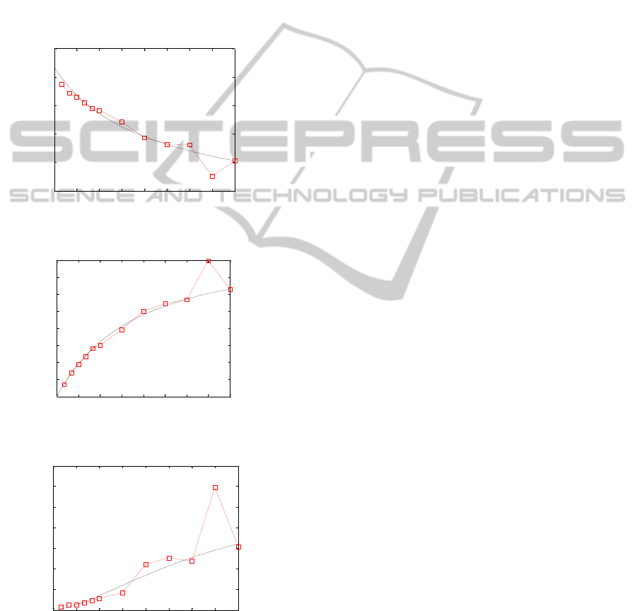
The system outputs and the sample are shown on

figures 1, 2 and 3 for hexadecane, spirits and

carbonyl compounds respectively.

0 1 2 3 4 5 6 7 8

3.5

4.5

5.5

Figure 1: Hexadecane concentration measurements and the

model output.

0 1 2 3 4 5 6 7 8

0.1

0.2

0.3

0.4

0.5

0.6

0.7

0.8

Figure 2: Spirits concentration measurements and the

model output.

0 1 2 3 4 5 6 7 8

0.2

0.4

0.6

0.8

1.2

1.4

Figure 3: Carbonyl compounds concentration

measurements and the model output.

As we can see on figures, the measurement at the

point

7t 

is an abnormal measurement, but it did

not effect on the model.

5 CONCLUSIONS

In this paper, the method of the ordinary differential

equation structure and parameters identification was

described. Within the proposed approach the system

structure and its parameters are automatically

determined. The suggested modifications of the

evolutionary strategies algorithm increase the

accuracy of model and allow solving two tasks at the

same time. The identification problem for

hexadecane disintegration reaction was considered.

Numerical experiments have demonstrated the

proposed approach usefulness.

The further investigation should be concentrated

on the estimation of the performance of algorithm

with the different local optimization and mutation

parameters.

REFERENCES

Janiczek T., Janiczek J., 2010. Linear dynamic system

identification in the frequency domain using fractional

derivatives. Metrol. Meas. Syst., Vol. XVII, No 2, pp.

279-288.

Parmar G., Prasad R., Mukherjee S., 2007. Order

reduction of linear dynamic systems using stability

equation method and GA. International Journal of

computer and Infornation Engeneering 1:1.

Romanovskii B. V., 2006. The foundations of the chemical

kinetics. Moscow: Ekzamen

Schwefel Hans-Paul, 1995. Evolution and Optimum

Seeking. New York: Wiley & Sons.

Zoteev V., 2008. Parametrical identification of linear

dynamical system on the basis of stochastic difference

equations. Matem. Mod., Vol. 20, No 9, pp 120-128.

The Application of Evolutionary Algorithm for the Linear Dynamic System Modelling

237