
Modeling Cell Populations in Development using Individual Stochastic
Regulatory Networks
Paweł Bednarz and Bartek Wilczy
´
nski
Institute of Informatics, University of Warsaw, Banacha 2, Warsaw, Poland
Keywords:
Stochastic Simulation, Cellular Population, Regulatory Network, GPU Computing.
Abstract:
We present a new approach to high level stochastic simulations of cell populations. The proposed method
employs the Stochastic Logical Network (SLN) method for simulating independent regulatory processes oc-
curring in individual cells allowing for efficient simulations of systems consisting of thousands of cells. The
stochastic logical network model is extended to account for not only regulatory control of gene expression
but other related processes such as: inter-cellular signaling, cell division and programmed cell death. In the
paper, we present the method and several case studies, where the proposed approach is used to provide models
of biological phenomena. These examples include community effect in gene expression, the role of negative
feedback in growing epithelial cell lineage and the role of asymmetric cell division in cell fate choices. We
present also an efficient implementation of the method using GPU computing and show that its performance
is significantly better than that using CPU.
1 INTRODUCTION
Modeling biological processes linked to gene regula-
tion is a very broad and diverse field. The problem is
fundamental and many different approaches with dif-
ferent advantages and disadvantages have been pro-
posed to address its various aspects (see (De Jong,
2002) for a review). In particular, development of
multi-cellular organisms presents many challenges as
it requires consistent models taking into account large
populations of cells able to perform their regulatory
programs independently but at the same time able to
communicate with each other via chemical signaling.
In addition, the developmental systems need to be ro-
bust to external conditions and at the same time, they
rarely operate under equilibrium conditions, requir-
ing models capable of capturing temporal behavior
as well as analysis of possible attractors and steady
states of the system. In addition, frequently possible
states of the system differ only by a small number of
molecules leading to stochastic behavior on a single-
cell level.
Boolean networks have been particularly useful
in modeling developmental systems (Thomas and
D’Ari, 1990), as they do not require exact rate con-
stants and they provide the modelers with models
which are relatively easy to study. However, most of
the systems are focusing on cell autonomous be-
havior, with notable exceptions of several exam-
ples of networks related to Drosophila segmentation
(S
´
anchez et al., 2008) or wing disc (Gonzalez et al.,
2008), however even those pioneering works have
only considered at most a handful of cells at once.
2 PROPOSED MODEL
We propose a new approach to modeling large cell
populations with explicitly simulating regulatory net-
works of each of the cells. The method is based on
stochastic logical networks (SLN), a generalization
of the Boolean network model which builds up upon
the non-deterministic state transitions in Boolean net-
works and defines a probabilistic model of state tran-
sitions. In the following sections we will briefly de-
scribe the SLN framework and how we use it for the
purpose of simulating cell populations.
2.1 From Boolean Networks to
Stochastic Logical Networks
Boolean networks have a long history of applications
to gene regulatory systems. Early work by Kauffman
(Kauffman, 1977) and Thomas (Thomas, 1978) led to
the representation of the regulatory network as a sys-
334
Bednarz P. and Wilczy
´
nski B..
Modeling Cell Populations in Development using Individual Stochastic Regulatory Networks.
DOI: 10.5220/0004060703340340
In Proceedings of the 2nd International Conference on Simulation and Modeling Methodologies, Technologies and Applications (SIMULTECH-2012),
pages 334-340
ISBN: 978-989-8565-20-4
Copyright
c
2012 SCITEPRESS (Science and Technology Publications, Lda.)

tem of Boolean equations. For example a simple neg-
ative feedback loop can be represented by two equa-
tions:
X ← Y
Y ← −X
In those first simple models of regulatory net-
works the dynamics was usually considered to be syn-
chronous, i.e. all genes changed their value to their
respective regulatory function (right-hand side of the
regulatory equation). While the simplicity of such an
approach might be appealing, it is now well known
that due to very different transcription and decay rate
for different genes, it is quite far from realistic.
Later, Thomas extended this formalism and pro-
posed generalized logical networks (Thomas and
D’Ari, 1990), which not-only introduced asyn-
chronous state change for different genes, but also
extended the state space to include more than two
expression levels for some of the genes. The asyn-
chronous state change had a major impact on the anal-
ysis of the system dynamics, as now instead of a sin-
gle successor state for any state of the network we had
to consider a set of possible successor states. While
it is clear that the asynchronous state transitions are
more realistic than synchronous, they also create chal-
lenges for the formal analysis of such systems as the
size of the state space visited from any initial state can
be much larger than in the synchronous case.
More recently, we proposed another extension
of the Generalized logic formalism, by introducing
stochastic models that could be built on top of the
generalized logical networks. Stochastic logical net-
works (SLN) (Wilczynski and Tiuryn, 2006) were
originally defined as continuous dynamical systems
with a canonical discretized form aimed at network
reconstruction from quantitative data (Wilczynski and
Tiuryn, 2007), however for the purposes of this arti-
cle, we will consider them to be discrete objects. Sim-
ilarly to the Boolean models, any SLN with N genes
consists of N variables g
1
, ..., g
N
each of which takes
values from a finite discrete set. For the purposes of
this article, we will consider only variables with bi-
nary value sets, but all the reasoning can be extended
to use variables with integer values and the proposed
implementation is ready to use such extended vari-
ables. The regulatory function of each gene g
i
is de-
scribed by an equation of the following form:
F
i
(g
1
, ..., g
N
) =
N
∑
j=1
w
ji
g
j
, (1)
where w
ji
is the regulatory influence of the gene g
j
on g
i
. For any state of the network, we can cal-
culate the regulatory function for each of the genes
F
i
= {F
1
, ..., F
N
}. Given the matrix W = {w
i j
}, SLN
model defines a probability distribution
R
i
(σ) =
|F
i
|
∑
|F
j
|
describing the probability of changing first the value
of gene i, given that we start from the state σ. Given
this probability distribution, we can employ an algo-
rithm, conceptually similar to the Gillespie’s stochas-
tic simulation method (Gillespie, 1977) to simulate a
cell behavior over time: in each step we select a gene
to change based on its total influence F
i
in comparison
to the total influence in the system.
2.2 Modeling Populations of Cells with
Stochastic Logical Networks
Starting with this slightly simplified definition of the
SLN model, we can extend it to systems consisting of
multiple cells with identical underlying genetic net-
work. To achieve this, instead of a single state σ, we
need to consider a population matrix P
i j
, where the i-
th row P[i] corresponds to a state of a single i-th cell.
With this representation, we can calculate the to-
tal influence of all genes by simply performing matrix
multiplication of P by the regulatory matrix W . Once
we have the influence, we just need to perform a sin-
gle step of the simulation for each of the cells in the
population to obtain the state of the population for the
next step.
To account for typical processes involved in gene
regulation in development, we have included addi-
tional actions performed at each step of population
simulation:
• There are special variables, regulated in the same
way as the gene variables, corresponding to the
cell division, and death. After calculating the state
of each cell, the algorithm checks whether the di-
vision or death variables are “active” and if it is
the case, it either removes the cell from popula-
tion or duplicates its row in case of symmetric di-
vision.
• For modeling signaling, a special vector is de-
fined for mapping each of the genes to secreted
molecules. Each secreted molecule is described
by a positive integer. If such value is placed on
the i-th position of the secretion vector and the i-th
gene is active, a predefined number of molecules
of the specified type is secreted to the environ-
ment. In case of non-secreted genes, the secretion
vector is set to 0.
• After the secretion is performed, another vector
mapping the signaling molecules back to genes is
ModelingCellPopulationsinDevelopmentusingIndividualStochasticRegulatoryNetworks
335
used. If the number of molecules of a given sig-
nal is non-zero, for each cell capable of receiving
such signal an integration event occurs randomly,
with the probability proportional to the number of
molecules divided by the number of cells in pop-
ulation.
This leads to the following algorithm:
Algorithm 1: Algorithm for a single step of STOPS simula-
tion.
Require: W : regulatory matrix
Require: P : population matrix
F ← P × W
for i=1 to N do
choose a random j according to distribution F
i
update P[i,j]
end for
for i=1 to N do
update Environment based on secretion from P[i]
end for
for i=1 to N do
update P[i] based on absorption from Environ-
ment
end for
for i=1 to N do
multiply or delete row P[i] based on special vari-
ables
end for
Using this algorithm, we can simulate any SLN
system provided that the matrix W , and the initial
population are specified. We have written a proto-
type implementation of this method called STOPS
(Stochastic Population Simulation) which is publicly
available on-line and was used to obtain the results
presented in the following section.
3 CASE STUDIES
In this section we describe three simple models of
small biological systems representative to questions
posed recently in the field of modeling regulatory
networks in development. Each of those examples
illustrates different capabilities of the STOPS mod-
eling framework. All presented examples were im-
plemented in STOPS and are publicly available for
download (see Sec. 6).
3.1 Community Effect in Gene
Expression
Recent study by Saka et al. (Saka et al., 2011) pro-
posed a simple model for the community effect in
gene expression occurring during embryonic develop-
ment of Xenopus frogs. During development, when it
is necessary to create continuous tissues in the em-
bryo it is usually achieved by formation of local ag-
gregates of cells with correlated expression of a cer-
tain gene by means of signaling. The community ef-
fect definition is based on the observation that while
such aggregates usually form around small foci of
cells initially expressing the identity factor of the de-
sired tissue, a certain number of cells capable of ex-
pressing this factor is required within the commu-
nity to achieve stable activation of the whole colony.
It was verified by dissection experiments, that if the
number of cells is below a certain threshold, the acti-
vation of all cells is unlikely, while above this thresh-
old the activation is prevalent among all cells.
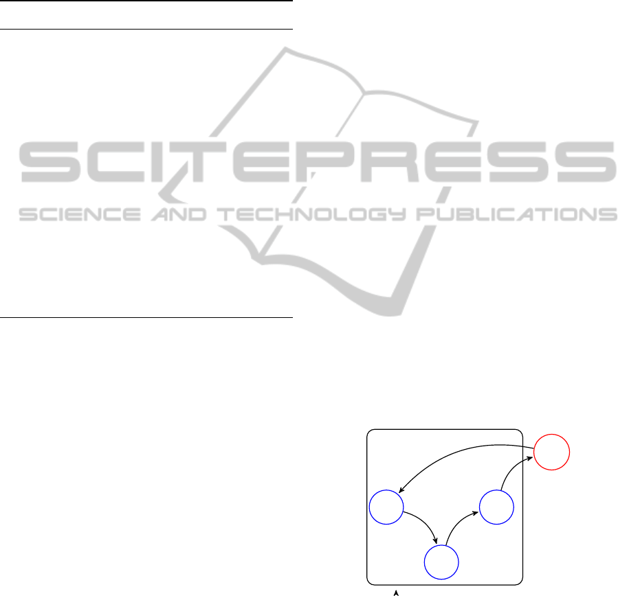
This system can be represented by a simple gene
network with signaling (see Fig. 1) as proposed by
Saka et al. (Saka et al., 2011). It includes the identity
gene g
1
, which is responsible for production of the
signaling molecule S, which is in turn secreted to the
environment and from there can be sensed by all other
cells via the receptor gene g
0
capable in turn of acti-
vating the identity gene g
0
. The whole network forms
a simple positive feedback loop responsible for ampli-
fying the initial signal, while the degradation rate of
the signaling molecule is responsible for the threshold
number of cells required for activation of majority of
cells.
Cell wall
g
0
g
1
S
Env
Figure 1: Simple gene regulatory network modeling com-
munity effect.
We have implemented this network in the STOPS
framework and performed one hundred simulations,
consisting of 30 steps each, for different colony sizes
ranging from 50 to 300 cells. Then we measured for
each of the trajectories, how many cells have the iden-
SIMULTECH2012-2ndInternationalConferenceonSimulationandModelingMethodologies,Technologiesand
Applications
336
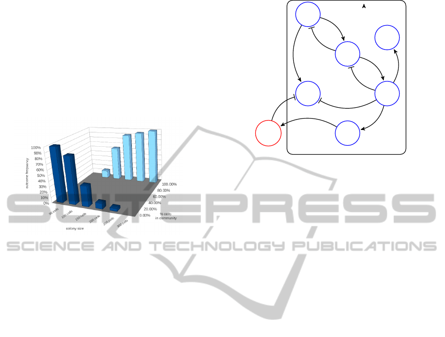
tity gene (g
1
) active as a fraction of the whole popula-
tion. For all cases, after 30 generations, we obtained
cell colony either fully activated or fully silent, which
is expected, given the presence of positive feedback
in the system. It was also reassuring to see that the
fraction of simulations leading to a fully activated sys-
tem is exhibiting a stepwise dependence on the colony
size: up to a 100 cells the silent case is clearly dom-
inant, while starting from 150 cells the active state is
dominating the results (see Fig. 2).
Figure 2: Outcomes of simulations of the community effect
model.
3.2 Linear Cell Lineage with
Proliferation
In a study by Lander et al. (Lander et al., 2009)
the authors consider a simple scenario where there
exists a pool of undifferentiated precursor cell pop-
ulation (expressing gene g
0
) which can then sponta-
neously switch to an intermediate differentiating state
(expressing g
1
) which then leads to the fully differ-
entiated terminal state (expressing g
2
). Importantly,
only the undifferentiated states (expressing g
0
or g
1
)
can divide, giving rise to new undifferentiated cells,
while the terminally differentiated cells (expressing
g
2
) can enter apoptosis (programmed cell death). The
system aims to model neural epithelia which consist
of similar types of cells, which are important for their
ability to quickly recover from removal of large num-
bers of differentiated and intermediate cells, provided
that they are left with enough pluripotent cells. Us-
ing an ODE model for this system, Lander et al. ob-
served that in order to achieve short recovery times
and limited total number of cells it is beneficial to pro-
vide negative feedback from the differentiated cells
instructing the pluripotent cells to limit their growth
rate when the number of differentiated cells is suffi-
cient.
Similar behavior can be observed in a system of
cells modeled with Stochastic Logical Networks fol-
lowing the genetic regulatory interactions depicted in
Figure 3. Each pair of genes representing consec-
Cell wall
g
0
g
1
g
2
S
Div
Env
Die
Figure 3: Gene network describing cell lineage with prolif-
eration and signaling.
utive cell stages is linked by direct negative feed-
back loop providing basis for cell progression through
the stages. There are two additional variables, cor-
responding to cell death and division and a signal-
ing molecule released by the terminally differentiated
cells and able to limit the proliferation of undifferenti-
ated cells receiving the signal. Gene g
2
corresponding
to the terminal differentiation is also activating cell
death and repressing proliferation.
To test whether the feedback cycle involving sig-
naling is required for the functioning of the system,
we can consider a system that is identical to the orig-
inal one, but does not include the signaling compo-
nent. Several exemplary trajectories of such a system
are shown in Figure 4. While the general behavior of
the system is consistent with earlier ODE simulations
by Lander and colleagues, it should be noted, that
the slope of recovery of the differentiated cells (blue
lines) is not as steep as it should be and that the re-
quired number of intermediate cells (green line reach-
ing 0.6 of the total population) are not supported by
the experimental data. It is also disturbing to see that
overall the population size is rapidly decreasing as a
result of very quick removal of the primary cells from
the population. It should be noted, that the problems
of the sub-population of proliferating cells extinction
is not visible in the original ODE model, as the pool
of non-differentiated cells can get arbitrarily close to
0 and still be able to regenerate, while our stochastic
model is capable of highlighting problems with mod-
els that lead to depletion of any sub-population as in
our model it is possible to consider parameters lead-
ing to a complete extinction of the system.
If we compare these results to the full model in-
cluding signaling to reduce proliferation when not
needed, we can see clear improvement (see Fig. 4
B). The number of intermediate cells stays below 30
ModelingCellPopulationsinDevelopmentusingIndividualStochasticRegulatoryNetworks
337
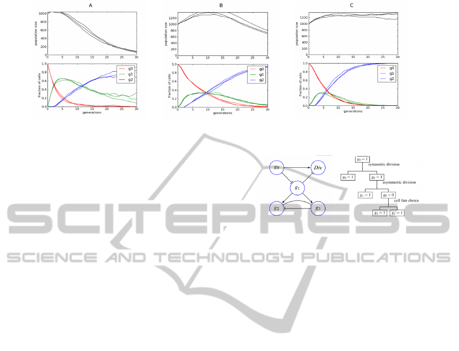
Figure 4: Results of simulation of the cell lineage without feedback (A), with simple feedback (B) and with cell-type specific
feedback (C).
per cent all the time and the decrease in the number of
primary cells is slower, however the regeneration rate
of the differentiated cells remains unchanged and the
population size problem is only slightly mitigated. So
while it is clear that including feedback in the system
improves the model, it is not sufficient to recapitulate
the experimental results (faster regeneration and sta-
ble population size). It turns out, that the reason for
these problems is the decreasing number of primary
cells and the difficulty of the ligand to find those cells
before being absorbed by the differentiated cells that
cannot respond to the signal as they are already un-
able to proliferate. This problem cannot be seen in
the ODE model, as there is dependence of the signal
reception by the relative proportion of dividing cells
in the population.
This problem can be eliminated by preventing the
differentiated cells from being able to receive signals
from the environment. Technically this can be done
by including another gene representing the receptor,
which is regulated by g
2
and which is necessary for
signal reception. Making this change to the system
gives much better results (see Fig. 4 C). Both prob-
lems: slow regeneration rate and population size in-
stability are solved making the model capable of re-
producing experimentally observed behavior.
3.3 Asymmetric Cell Division and
Cell-fate Choice
While signaling is a very powerful mechanism of con-
trolling state changes in developing cells, it is fre-
quently the case that the cell fate choice is determined
by other mechanisms. Cohen et al. (Cohen et al.,
2010) studied recently a system of neural cells dif-
ferentiation, which includes two such mechanisms:
asymmetric cell division and spontaneous stochastic
cell-fate choice based on a bistable system of two
genes.
The asymmetric division is a mechanism in which
a cell expressing a pluripotency factor (in this case
Figure 5: Network model of cell-fate choice with asymmet-
ric cell division and the associated cell lineage tree.
a gene called “numb”) is undergoing an asymmetric
division resulting with one of the daughter cells re-
taining majority of the factor protein, while the other
daughter cell is born free of this protein. This leads
these two cells to reach different regulatory states,
since the pluripotency factor is lost in one of the re-
sulting cells allowing it to start the differentiation pro-
cess. On the regulatory level, the pluripotency factor
is usually a repressor of the differentiation factors. In
case of numb, it represses notch which is responsi-
ble for facilitating specification of cells into neurons
(Shen et al., 2002).
The stochastic cell-fate choice facilitated by a
bistable switch is a different regulatory mechanism
which allows cells that already started differentiation
to commit stably to one of the predefined cell-fates.
It is nicely illustrated by the gene regulatory net-
work for Arabidopsis flower development (Espinosa-
Soto et al., 2004), where undifferentiated cells need to
commit to one of the four cell-fates to make all neces-
sary parts of the flower. On the regulatory level, such
system, in its most basic form, consists of an initial
signal: the differentiation factor which drives the ex-
pression of two, mutually exclusive, terminal cell-fate
genes. Both these genes are repressing each other and
repressing the upstream signal leading to the system
with two attractors with either one (and only one) of
the cell-fate genes on.
The system studied by Cohen and colleagues con-
sisted of both those components: first it had undif-
ferentiated cells capable of either self-reproduction
by symmetric divisions or performing an asymmetric
division leading to creation of a differentiating cell
SIMULTECH2012-2ndInternationalConferenceonSimulationandModelingMethodologies,Technologiesand
Applications
338
which could then choose one of the two predefined
cell fates. Interestingly, the authors provided exper-
imental measurements of relative number of events
leading to the symmetric vs. asymmetric divisions (53
vs. 19 respectively) and of the relative frequencies of
choosing different cell-fates (10 vs 16). This allowed
us to attempt to build a model capable of reproducing
this behavior using the STOPS framework.
The regulatory network we designed is presented
in Figure 5. It consists of the pluripotency factor g
0
repressing the differentiation factor g
1
, which has a
basal expression level driving its expression immedi-
ately upon loss of g
0
. Naturally, the proliferation fac-
tor activates the capability of cells to proliferate, while
the differentiation gene is shutting this program down
upon activation. The asymmetric division is acting on
the expression level of g
0
: assuming that the parent
cell had the gene on an asymmetric division results
with two cells which are identical to the parent cell
regarding all genes but g
0
which will be on in one of
the daughters and off in the other.
Once the differentiation factor g
1
is turned on, it
starts driving the expression of both cell fate genes,
however it is not necessarily acting on both of them
with the same regulatory influence. In fact making
those influences different is essential for reproduc-
ing the correct ratio between the numbers of different
cell-fates in resulting population. At some point, one
of the target gene gets activated subsequently leading
to stable repression of the alternative cell fate. The
overall cell-fate choice diagram is shown in Figure 5
(B).
The results of the simulation are capturing the
general behavior of the system and by choosing the
regulatory influences carefully, we were able to ob-
tain simulation results matching the experimental re-
sults published by Cohen et al. (Cohen et al., 2010).
4 IMPLEMENTATION AND
PERFORMANCE
BENCHMARKS
The first prototype of our stochastic population sim-
ulation (STOPS) method was implemented in pure
python scripting language. While it was convenient
for the prototype, the performance of such a solution
was far from satisfactory. Since this tool is intended
to be used for simulation of cellular populations with
realistic sizes it needs to be able to tackle meaningful
time-scales (thousands of simulation steps) for popu-
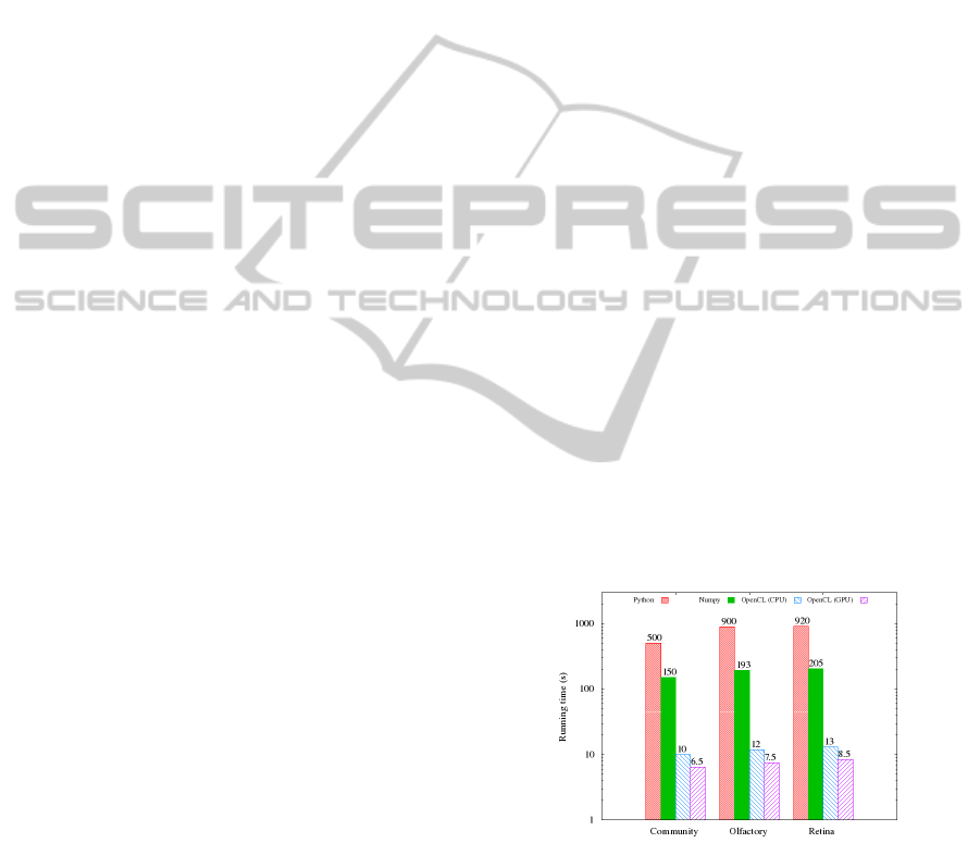
lations consisting of millions of cells. As we can see
in Figure 6, the prototype implementation requires be-
tween 10 and 15 minutes for a single simulation step
for a population of 10 million cells.
In order to provide a more efficient platform for
realistic simulations, we have re-implemented the
main algorithm in two different libraries dedicated
to matrix operations: NumPy (Harrington and Gold-
smith, 2009) and pyOpenCL (Kl
¨
ockner et al., 2012).
The first one has the advantage of being available on
all major platforms, making it possible for anyone to
install STOPS on their machine and test it with rea-
sonable efficiency. The second implementation uses
the OpenCL bindings and allows users equipped with
a machine with a support for an OpenCL implemen-
tation (currently there are OpenCL implementations
released for AMD and Intel CPUs as well as Nvidia
and ATI GPUs) to take advantage of the full poten-
tial of their hardware. We have tested the perfor-
mance of all three implementations on a computer
equipped with an Intel Xeon 3.2Ghz CPU and an
Nvidia Tesla C1070 GPU. It is clear from Figure 6
that while all three implementations taking advantage
of specialized matrix algebra operations outperform
the initial version by an order of magnitude, it should
be noted that the OpenCL version is still an order of
magnitude faster than the NumPy version. Interest-
ingly, the OpenCL performs similarly well both on
CPU and GPU implementations of the OpenCL li-
brary. It is important, as the CPU has typically access
to much larger memory, allowing for simulations of
much larger systems. It should be noted that the mem-
ory consumption is the same (number of cells times
the number of variables times the size of an integer).
Figure 6: Comparison of running times for different STOPS
implementations on three case-study datasets.
5 DISCUSSION AND FUTURE
WORK
We presented here a new approach to modeling cell
populations using stochastic logical networks. It
is particularly well suited for developmental sys-
ModelingCellPopulationsinDevelopmentusingIndividualStochasticRegulatoryNetworks
339

tems, where stochastic behavior of large populations
of proliferating and signaling cells is driven by the
same underlying regulatory machinery encoded in the
genome. We also provide a prototype implementa-
tion capable of simulating cell populations with mil-
lions of cells on a standard personal computer. Even
though the method is rather simple and requires only a
handful of parameters to run a simulation, it is able to
reproduce the results of many more established meth-
ods for wide variety of models relevant for problems
currently under consideration by the modeling com-
munity. In some cases, like the linear cell lineage sys-
tem, it can give us new insights missed by the ODE
model due to its more accurate representation of small
cell populations.
While the results shown are promising, the imple-
mentation is still in an early phase and could greatly
benefit from multiple improvements. One key area
that will work on in the future is extending the model
to take into account spatial aspect of cell populations.
Such functionality would greatly expand the range of
possible applications of this model, however mod-
eling spatially variable signalling without great de-
crease in the method performance poses a consider-
able challenge.
6 AVAILABILITY
The STOPS (STOchastic Population Simulation)
software implementation is publicly available under
the GNU GPL v.2 license. The implementation of all
three case studies is included in current version avail-
able at http://launchpad.net/stops.
ACKNOWLEDGEMENTS
This work was partially supported by the Polish Min-
istry of Science and Education grant number N N301
065236 and by the Foundation for Polish Science
within Homing Plus programme co-financed by the
European Union - European Regional Development
Fund.
REFERENCES
Cohen, A., Gomes, F., Roysam, B., and Cayouette, M.
(2010). Computational prediction of neural progen-
itor cell fates. Nature Methods, 7(3):213–218.
De Jong, H. (2002). Modeling and simulation of genetic
regulatory systems: a literature review. Journal of
computational biology, 9(1):67–103.
Espinosa-Soto, C., Padilla-Longoria, P., and Alvarez-
Buylla, E. (2004). A gene regulatory network
model for cell-fate determination during Arabidopsis
thaliana flower development that is robust and recov-
ers experimental gene expression profiles. The Plant
Cell Online, 16(11):2923.
Gillespie, D. (1977). Exact stochastic simulation of coupled
chemical reactions. The journal of physical chemistry,
81(25):2340–2361.
Gonzalez, A., Chaouiya, C., and Thieffry, D. (2008). Logi-
cal modelling of the role of the hh pathway in the pat-
terning of the drosophila wing disc. Bioinformatics,
24(16):i234–i240.
Harrington, J. and Goldsmith, D. (2009). Progress report:
Numpy and scipy documentation in 2009. In Varo-
quaux, G., van der Walt, S., and Millman, J., editors,
Proceedings of the 8th Python in Science Conference,
pages 84 – 87, Pasadena, CA USA.
Kauffman, S. (1977). Gene regulation networks: A theory
for their global structure and behaviors. Current topics
in developmental biology, 6:145–182.
Kl
¨
ockner, A., Pinto, N., Lee, Y., Catanzaro, B., Ivanov,
P., and Fasih, A. (2012). Pycuda and pyopencl: A
scripting-based approach to gpu run-time code gener-
ation. Parallel Comput., 38(3):157–174.
Lander, A., Gokoffski, K., Wan, F., Nie, Q., and Calof, A.
(2009). Cell lineages and the logic of proliferative
control. PLoS Biology, 7(1):e1000015.
Saka, Y., Lhoussaine, C., Kuttler, C., Ullner, E., and Thiel,
M. (2011). Theoretical basis of the community effect
in development. BMC Systems Biology, 5:54.
S
´
anchez, L., Chaouiya, C., and Thieffry, D. (2008). Seg-
menting the fly embryo: logical analysis of the role of
the segment polarity cross-regulatory module. Int. J.
Dev. Biol, 52(8):1059–1075.
Shen, Q., Zhong, W., Jan, Y. N., and Temple, S. (2002).
Asymmetric numb distribution is critical for asym-
metric cell division of mouse cerebral cortical stem
cells and neuroblasts. Development, 129:4843–4853.
Thomas, R. (1978). Logical analysis of systems compris-
ing feedback loops. Journal of Theoretical Biology,
73(4):631–656.
Thomas, R. and D’Ari, R. (1990). Biological feedback.
CRC press.
Wilczynski, B. and Tiuryn, J. (2006). Regulatory network
reconstruction using stochastic logical networks. In
proceedings of the Computational Methods in Systems
Biology 2006, Lecture Notes in Bioinformatics, pages
142–154. Springer Verlag.
Wilczynski, B. and Tiuryn, J. (2007). Reconstruction of
mammalian cell cycle regulatory network from mi-
croarray data using stochastic logical networks. In
proceedings of the Computational Methods in Systems
Biology 2006, Lecture Notes in Bioinformatics, pages
121–135. Springer Verlag.
SIMULTECH2012-2ndInternationalConferenceonSimulationandModelingMethodologies,Technologiesand
Applications
340
