
Linear Software Models for Well-composed Systems
Iaakov Exman
Software Engineering Dept., Jerusalem College of Engineering, POB 3566, Jerusalem, 91035, Israel
Keywords: Software Composition, Linear Software Models, Well-composed Systems, Modularity Matrix, Linear-
Reducible Matrix.
Abstract: Modularity is essential for automatic composition of real software systems from ready-made components.
But given ready-made components do not necessarily correspond exactly to the units and functionality of
designed software system architecture modules. One needs a neat composition procedure that guarantees the
necessary and sufficient components to provide required units. Linear Software Models are rigorous
theoretical standards subsuming modularity. The Linear-Reducible model is proposed as a model of well-
composed software systems, above and beyond software variability. Indeed, case studies of representative
systems recognized as well-composed, be they small, intermediate building blocks or large scale, are shown
to be Linear-Reducible. The paper lays down theoretical foundations – upon exact linear independence and
reducible matrix concepts – providing new precise meanings to familiar modularity ideas, such as the single
responsibility theorem. The theory uses a Modularity Matrix – linking independent software structors to
composable software functionals in a Linear Model.
1 INTRODUCTION
Significant progress since Parnas’ classical paper
(Parnas, 1972) – which posed the modularity issue in
the software context and treated it by informal
reasoning – paved the way for automatic run-time
system composition/update from ready-made
software components. Yet there remain fundamental
obstacles to make this vision concrete.
Modularity’s wisdom of low dependency among
modules has been informally stated in innumerable
ways: recommendations such as single
responsibility, source-code dependency metrics,
design patterns and tools. But recommendations,
metrics, patterns and tools never crystallized into a
systematic theoretical approach.
This is exactly the problem dealt with by this
paper: to provide a solid and generic basis to treat
software composition in a rigorous and consistent
way, enabling theoretical models against which to
check real systems. To this end, Linear Software
Models are proposed upon well-established linear
algebra techniques.
1.1 The Software Composition
Problem
The software composition problem, analysed by this
paper, is how to build a well-designed modular
software system from available ready-made
components that were not designed specifically for a
particular system.
Components are deployment units needed to
actually run software systems. They are loaded to
the computer memory as indivisible wholes. Typical
examples are a C++ dll (dynamically linked library),
a jar (Java archive) or a C# assembly.
On the one hand, the software engineer, by using
best practices, designs a modular software system in
terms of desirable architectural units. Architectural
units describe the structure and behaviour of a
particular software system.
On the other hand, components are assumed to
be mainly purchased as COTS (Commercial Off-
The-Shelf) components from several manufacturers,
and less frequently to be produced in-house. It is
realistic to expect variability among COTS from
distinct sources.
92
Exman I..
Linear Software Models for Well-composed Systems.
DOI: 10.5220/0004085500920101
In Proceedings of the 7th International Conference on Software Paradigm Trends (ICSOFT-2012), pages 92-101
ISBN: 978-989-8565-19-8
Copyright
c
2012 SCITEPRESS (Science and Technology Publications, Lda.)
1.2 Linear Software Models: Structors
and Functionals
This paper describes Linear Software Models as a
theory of software composition. In this theory, the
architecture of a software system is expressed by
two kinds of entities: structors and functionals.
Structors – a new term reminding vectors – are
architectural units, from the structural point of view.
Structors generalize the notion of structural unit to
cover diversity of types (structs, classes, interfaces,
aspects) and hierarchical collections (sets of classes,
as design patterns). Structors refer to types, not
instances. Structors are loadable within components.
Functionals are architectural system units from a
behavioural point of view. These are potential
functions that can be, but are not necessarily
invoked. Typically these are Java or C# methods,
related functions (e.g. a set of trigonometric
functions) or roles – supplying the functionality of a
design pattern (Riehle, 1996). Note: we use
Functional as a noun, similarly to the mathematical
concept with this name in the calculus of variations,
and to the grammatical use of Potential in physics.
Structors in general contain a finite set of
functionals and are represented by finite vectors.
Modules are architectural units in a higher
hierarchical level of a system. Modules are
composed of grouped structors and their
corresponding functionals.
Both components and systems contain structors.
But the respective logics are different. Structors
contained in a COTS component are fixed by the
core technology of the component manufacturer and
such structors must be assumed indivisible.
Structors within a system are determined by the
software system purpose. Thus, not all structors of a
component may be required by a system. Similarly,
not all functionals provided by structors are needed
by a system, and some of them may never be
invoked. The numbers of structors or functionals
provided by a component are not constrained.
Analysis starts with a list of structors and a list of
functionals that must be in a system. If two structors
provide distinct functionals, both are needed. If they
provide the same functionals, one of them is
redundant. For partial overlap, either one may be
complemented by a third structor. But which one is
preferable? Within a Linear Software Model the
answer is clear: choose a linearly independent set of
structors.
Linear models are usually formulated in terms of
matrices. The Modularity Matrix is a Boolean matrix
with columns standing for structors and rows for
functionals. A matrix element is 1-valued for a
functional-structor link and 0-valued for no link.
1.3 Modularity Matrix: An
Introductory Example
A simple yet useful system is here described in
terms of a Linear Software Model to illustrate
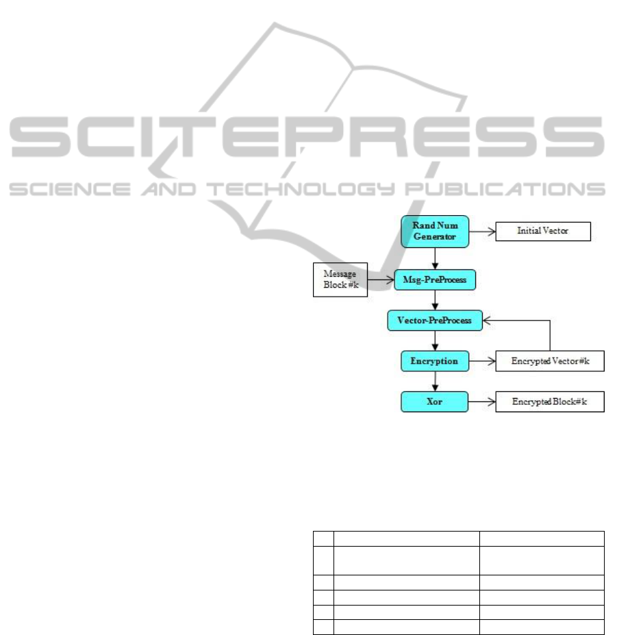
concepts found along the paper. It refers to OFB
(Output Feed-Back) encryption of a long message
(Fig. 1) before network transmission – e.g.
(Kaufman, et al. 1997). A message is cut into N
blocks of fixed length and each one is treated
separately.
A random number, the Initial Vector, is
generated. Each block of the message is pre-
processed. A corresponding vector is also pre-
processed to be of the size of a block, and then
encrypted. The encrypted output vector is fed back
into the encryption function, through the vector pre-
processing. Feedback is done N times, obtaining one
vector for each message block. The k
th
encrypted
vector is then Xored with the k
th
message block.
Figure 1: OFB encryption of long message. This is a
functional calling dependency graph for a generic k
th
message block. Functionals are displayed as (blue)
rounded rectangles. Some of the input/output dataflow is
shown in regular rectangles.
Table 1: OFB Functionals.
#
Functional
Description
1
Random number
generator
from a distribution
2
Encryption function
e.g. RSA encryption
3
Xor
a logical function
4
Vector-Pre-Process
Fetch(vector,size)
5
Message-Pre-Process
fetch & pad message
The OFB software system has five functionals
(Table 1) and the following four structors: S1) Rand
- offers random distributions; S2) Crypto structor -
Linear Software Models for Well-composed Systems
93
offers encryption protocols; S3) Logical - provides
logical functions, say AND, OR, XOR; S4) Proc - a
processor structor provides pre-processing functions.
The resulting OFB modularity matrix (Table 2)
has 2 identical lowest rows. The matrix reflects that
the pre-processing functionals are not independent.
Both functionals are provided by the same structor,
thus they are not distinguishable.
Table 2: OFB Rectangular Modularity Matrix with Linear
Dependencies.
S1=Rand
S2=Crypto
S3=Logical
S4=Proc
Rand Num Gen
F1
1
0
0
0
Encryption Func
F2
0
1
0
1
XOR
F3
0
0
1
1
Vector-Pre-Proc
F4
0
0
0
1
Msg-Pre-Proc
F5
0
0
0
1
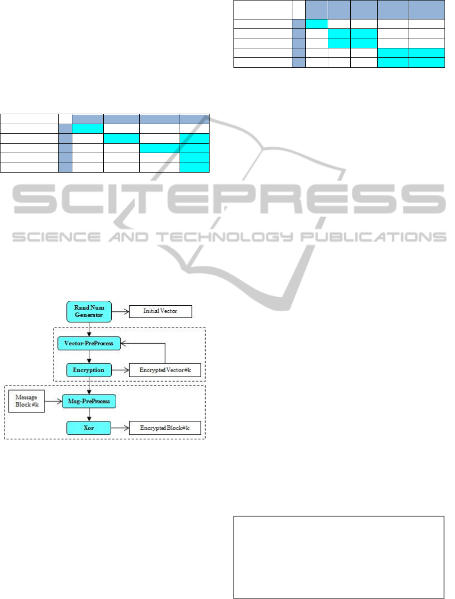
An interesting feature of OFB encryption is that
one can prepare all encrypted vectors in advance,
before there are any message blocks to be sent.
Therefore, one can rearrange the functional calling
graph, enabling totally separate execution.
Two modules naturally appear, one dealing with
vectors and the other with message blocks – see Fig.
2. In each module, the processing structor, besides
pre-processing, invokes the respective processing
functional.
Figure 2: OFB functionals modularized. Rearranged
functional calling dependency graph for a generic k
th
message block. The upper dashed lines module pre-
processes vectors, encrypts and saves them. The lower
module fetches message blocks, pre-processes them and
Xors each message block with its saved vector. This figure
uses the same conventions as the previous figure.
Independent pre-processing functionals which
are able to run in parallel in distinct machines need
independent structors. So, one has a VectorProc
structor and a separate MsgProc structor. These
structors are aware – by means of associations – of
the respective processing functionals which they are
able to invoke.
Table 3: OFB Strictly Linear Model – Modularity Matrix.
S1=
Rand
S2=
Crypt
S4=Vec
Proc
S3=
Logical
S5=Msg
Proc
Rand Num Gen
F1
1
0
0
0
0
Encryption Func
F2
0
1
1
0
0
Vector-Pre-Proc
F3
0
0
1
0
0
XOR
F4
0
0
0
1
1
Msg-Pre-Proc
F5
0
0
0
0
1
Row and column swap operations lead to a
block-diagonal matrix (Table 3). The diagonal
blocks in this matrix match the modules in Fig. 2.
The system matrix in Table 3 strictly obeys a
Linear Software Model. This means that all its
modules have linearly independent rows and
columns. Thus, each of its functionals is
distinguishable. For instance, according to the
matrix in Table 3 functional F
2
is provided by
structors {S
2
, S
4
}.
The independent execution of VectorProc and
MsgProc, in time and space, clarifies the sense of an
independent software structor. It must be: a)
Loadable/Runnable – in a virtual or real machine; b)
Separable – i.e. able to run in separate machines.
The remaining of the paper is organized starting
from the basic theory (section 2), through concrete
case studies (section 3), to a discussion (section 4).
2 LINEAR SOFTWARE MODELS
OF COMPOSITION
The aim of this section is to describe the new
theoretical approach – the Linear Software Models
of Composition.
Linear Software Models are the simplest
theoretical models of software composition. Systems
obeying such a model are composed just by addition
of independent modules.
2.1 Modularity Matrices’ Linear
Independence
A Linear Software Model contains a list of software
structors and another of software functionals. Its
Modularity Matrix is defined as:
Definition 1 – Modularity-Matrix
A fully expanded Modularity-Matrix is a
Boolean matrix asserting links (1-valued
elements) between software functionals (rows)
and software structors (columns). The absence
of a link is marked by a 0-valued element.
ICSOFT 2012 - 7th International Conference on Software Paradigm Trends
94

By definition, software structors are elementary
artifacts, which the software engineer decides to
look at them as indivisible into smaller structors.
Say, the OFB crypto structor (section 1.3) is not split
into – prime factorization or modulo arithmetic –
although decomposition is obviously possible. The
same holds true for functionals.
Besides being indivisible, only structors with
unique roles, as the OFB VectorProcessor and
MsgProcessor needed for parallelism, are in the
Matrix. Multiple structor copies, say by fault
tolerance reasons, are not included in the Matrix.
Independent structors must be represented by
distinct vectors. But, sets of differing vectors may
still be dependent. The generic criterion for
independent structors in any system subsets is linear
independence:
We now look at the links from the functional
point of view. In order to be able to distinguish a
functional, its set of links in the functional row must
be unequivocal. Again linear independence is the
relevant criterion:
For instance, for OFB (Table 3) the XOR
functional composition set is {S3, S5}.
2.2 Well-composed Modularity
Matrices are Square
A well-composed modularity matrix has additive
properties, i.e. it has composable functionals from
independent structors. Then:
A proof sketch is (detailed proofs will be given
in a long paper): Assume a matrix without empty
rows/columns. First, structors are used as a basis for
functional vectors. Then, functionals are a basis for
structor vectors. By linear independence, in each
case vector numbers cannot be greater than the basis.
As both cases must be simultaneously true, follows
the equality N
S
=N
F
. The matrix is square.
The theorem assumptions are very intuitive. An
analogy is the symptom sets to diagnose illnesses.
Say, high temperature, a very common symptom, is
not enough to identify a disease. Diseases with the
same symptom sets are indistinguishable. To
unequivocally diagnose an illness one needs
independent sets of symptoms.
This theorem does not force a one-to-one
functional/structor match. It is obeyed by matrices
with N
VAL
1-valued elements greater than N
S
and N
F
(see e.g. Table 4).
Table 4: Abstract square Modularity Matrix with
NVAL=6, while NS=NF=3.
S1
S2
S3
F1
1
0
1
F2
0
1
1
F3
1
1
0
Algebraically, there are simple criteria for well-
composed matrices: non-zero matrix determinant or
matrix rank equal to the number of rows/columns.
2.3 Reducible Modularity Matrices
When a Modularity Matrix has disjoint dependency
sets, structors and their functionals can be grouped
into modules, such that vector sets in different
modules are linearly independent. This reduces the
matrix to block-diagonal (fig. 3), i.e. with smaller
squares of any size along the diagonal (Rowland,
Weisstein, 2006). All off-block elements are zero.
Definition 2 – Independent Structor
A software structor is independent of other
structors in the system, if it provides a non-
empty proper sub-set of functionals of the
system, given by the 1-valued links in the
respective column, and is linearly independent
of other columns in the Modularity Matrix.
Definition 3 – Composable Functional
A software functional is independently
composable or just composable in terms of
structors, if it corresponds to a non-empty
proper sub-set of system structors, given by the
1-valued links in the respective row, and is
linearly independent of other rows in the
Modularity-Matrix.
This set is the composition set of the functional.
Theorem 1 – Well-Composed Modularity-
Matrix
If in a Modularity-Matrix all its functionals are
composable with independent structors, the
Modularity-Matrix number of structors N
s
is
equal to its number of functionals N
F
. The
matrix is Square.
Such a matrix is called a Well-Composed
Modularity-Matrix.
Linear Software Models for Well-composed Systems
95
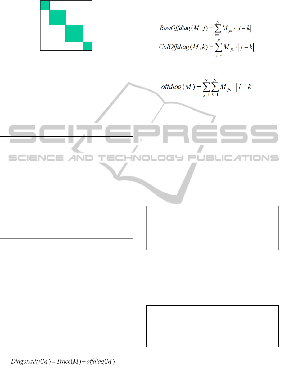
Figure 3: Schematic Block-Diagonal Matrix.
A “union-set” is the union of composition sets
for a set of functionals. Then:
A proof sketch is: apply row and column
exchanges to bring the disjoint union-set to the
upper-left matrix corner. As the whole Modularity
Matrix is Well-composed, the disjoint union-set is
itself square (by Theorem 1) and its diagonal is
along the whole Matrix diagonal. The residual 1-
valued elements are thus also square bounded, along
the whole Matrix diagonal. This reasoning is
extensible to any number of blocks.
The previous theorems naturally lead us to define
linear software system models of composition. The
two theorems are combined in the Linear-Reducible
model, in the strict sense.
We identify modules with disjoint diagonal
blocks of structors/functionals, corresponding to the
intuitive notion of modular software systems. One
can express modularity quantitatively by the
diagonality of a Modularity-Matrix M, telling how
close its 1-valued elements are to the main diagonal.
It is the difference between the Trace, the diagonal
elements' sum, and offdiag, a new term dealing with
off-diagonal elements:
(1)
Offdiag sums over 1-valued M
jk
off-diagonal
elements, times the absolute value of the difference
of the element’s column k and row j indices. For
each row j and column k:
(2)
The overall matrix offdiag is:
(3)
The next operations may unfold a whole
hierarchy of block levels, where a level is defined by
the matrix components explicit in that level:
a- Block collapse – transforms a block into a
single element black-box.
b- Block expansion – restores a collapsed black-
box back into a white-box.
To assure that these operations preserve
diagonality, black-boxes are labeled by the <Trace,
offdiag> diagonality value, of the original white-
box. To be able to restore the white-box, hidden
rows/columns should be stored elsewhere.
The modularity hierarchy is thus given by:
2.3 The Single Responsibility Theorem
The last theoretical piece of the Linear Models is a
linear algebraic formulation of the single
responsibility principle (Martin, 2003). It is valid
after one obtains a block-diagonal matrix:
This theorem is easily verified. It means that a
single module is responsible for providing each
functional exclusively by its structors. This is a
plausible interpretation of the familiar principle,
Theorem 2 – Modularity Matrix Reducibility
Any well-composed Modularity Matrix in which
the union-set for a given set of functionals is
disjoint to the other functional union-sets is
reducible, i.e. it can be put in block-diagonal
form.
Definition 4 – Linear Reducible Model
The Linear-Reducible model of software system
composition, in the strict sense, is characterized
by a well-composed and reducible Modularity
Matrix having at least two disjoint blocks.
Definition 5 – Number of modules at a level
The number of modules
of a software system at a
hierarchy level is the number of blocks from the
modularity matrix partition into disjoint union-
sets at that level.
Theorem 3 – Single Responsibility
In a strictly block-diagonal modularity matrix
each structor column intersects a single module.
Similarly, each functional row intersects a single
module.
ICSOFT 2012 - 7th International Conference on Software Paradigm Trends
96
since related structors and functionals are grouped in
a single module.
3 CASE STUDIES
The goal of this section is to demonstrate the power
of Linear Software models, showing by case studies
a range of concrete software systems obeying such a
model.
We have chosen representative software systems
of disparate purposes and sizes to illustrate the
Linear Models. It turns out that all systems are well-
composed. Small systems are strictly Linear-
Reducible – i.e. obey a model with a linearly
independent and reducible matrix – and larger
systems are bordered Linear-Reducible. In each
case, a modularity matrix is obtained, block-
diagonalized and analysed in terms of Linearity.
3.1 Small Systems are Strictly Linear
Reducible
Small systems and intermediate reusable building
blocks strictly obey the Linear-Reducible Software
model. These are Parnas’ KWIC index and the
Observer pattern. KWIC was thoroughly analysed
by Parnas to be a canonical example. The Observer
pattern was deliberately designed to be reused.
3.1.1 Parnas' KWIC Index
The 1972 Parnas paper (Parnas, 1972) described two
KWIC index modularizations. The system outputs
an alphabetical listing of all circular shifts of all
input lines. Functionals were extracted from Parnas’
own system description. Structors are explicit in the
paper – where they are called modules.
The Modularity Matrix of Parnas’ 1
st
modularization is in Table 5 (0-valued elements are
omitted for clarity; blocks have a darker
background). It is almost block-diagonal, but two
features are problematic:
a- the Master Control column vector is not a
proper subset of the functionals;
b- non-zero outliers break block-diagonality.
The matrix clearly hints to couplings to be
resolved: the notably higher RowOffdiag=4 of the 3
rd
row, contains all outliers, besides the master control
ones. The solution is: a- to delete the master control,
as quoting Parnas, it “does little more than
sequencing”, it is not a real structor; b- to add a new
Line-Storage structor, as Parnas informally argued,
Table 5: Parnas' 1
st
Modularization – Modularity Matrix.
Structors
Input
Circular
Shifter
Master
Control
Alpha-
betizer
Output
Functionals
1
2
3
4
5
Input = ordered set of lines
1
1
1
Does circular shift on a line
2
1
1
Line= store line in word order
3
1
1
1
1
Sort lines in alphabetical order
4
1
1
Outputs circular shifted lines
5
1
1
to decouple the 3
rd
row "Line" functional from the
Input, Circular-shifter and Alphabetizer. The 2
nd
Parnas’ modularization fits the strictly diagonal 5-
module matrix in Table 6.
Table 6: Parnas' 2
nd
Modularization – Modularity Matrix.
Structors
Input
Circular
Shifter
Line
Storage
Alpha-
betizer
Output
Functionals
1
2
3
4
5
Input = ordered set of lines
1
1
Does circular shift on a line
2
1
Line= store line in word order
3
1
Sort lines in alphabetical order
4
1
Outputs circular shifted lines
5
1
We use decouple in a precise new meaning, of
enabling linearly independent composition.
The matrices in Tables 5 and 6 are not
equivalent, having different non-zero element
numbers. Which one is more modular? The 1
st
matrix diagonality has a value –5. The 2
nd
diagonality equals the Trace and is 5. Thus, the 2
nd
is
more modular.
We arrived at the same Parnas conclusions, by
formal Modularity Matrix arguments. This system
strictly obeys the Linear-Reducible Model.
3.1.2 Observer Design Pattern
The Observer Design Pattern abstracts one-to-many
interactions among objects, such that when a
"subject" – changes, all the "observers" – are
notified and updated.
The Observer Modularity Matrix is based upon
the Design Patterns’ GoF book (Gamma, et al.,
1995). Its sample code refers to an analog and a
digital clock, the "concrete observers", changing
according to an internal clock – the "concrete
subject".
The system structors (Table 7) are:
generic Observer pattern entities, directly
taken from the pattern list of “Participants”;
(the first four rows of Table 7).
specific application structors – a subject
resource, a GUI for each external clock and
an initiator which constructs the clocks.
Linear Software Models for Well-composed Systems
97
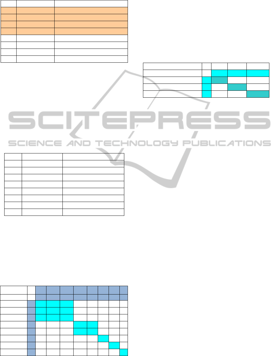
Table 7: Observer - Structors.
Structors
Description
1
abstract subject
interface to attach/detach observers
2
abstract observer
interface to update an observer
3
concrete subject
stores global state; sends notifications
4
concrete observer
implements the observer updating
5
subject resource
internal timer ticks the global state
6
analog GUI
inherits graphics analog clock widget
7
digital GUI
inherits graphics digital clock widget
8
initiator
to construct the clock objects
The Observer functionals were extracted from
the complete set of functions that may be invoked in
the sample code. These functions were trimmed by
elimination of linear dependencies.
State is not maintained in the same way in the
subject and in the observers. The unique subject sets
the state ("ticks") by means of a Keep-Global-state
functional, while observers, are updated at unrelated
times and Keep-Local-state. Table 8 shows the
Observer functionals.
Table 8: Observer – Functionals.
Functionals
Description
1
Keep-observers-list
attaching/detaching observers
2
Notify observers
notify when subject changes
3
Update observers
update observers, after notify
4
Keep-Global-state
keep time to allow updates
5
Keep-Local-state
keep time in each observer
6
Draw-analog
specific analog clock draw
7
Draw-digital
specific digital clock draw
8
Constructor
construct the clock objects
Row/column reordering of a quite arbitrary
initial matrix causes modules to emerge in a strictly
Linear-Reducible matrix. (Table 9). These modules
are a subject and an observer – the generic module
roles (Riehle, 1996) for this design pattern – each
one with the respective abstract/concrete structors,
and the specific clock application modules.
Table 9: Observer Linear Reducible – Modularity Matrix.
Structors
subject
concrete
subject
subject
resource
concrete
observer
Obser
ver
Gui
analog
Gui
digital
Init
Functionals
1
2
3
4
5
6
7
8
Keep observer list
1
1
Notify observers
2
1
1
Keep-global-state
3
1
1
Keep-local-state
4
1
Update observers
5
1
1
Draw-analog
6
1
Draw-digital
7
1
Constructor
8
1
In Table 9, subject and observer modules
emerged from basic structors. Alternatively one can
deal with black-box collapsed modules (as defined
in sub-section 2.3) in a higher hierarchical level
matrix shown in Table 10.
In either format, one could analyse the pattern
matrix (subject and observer) as a generic building
block in separate from the specific clock application.
Table 10: Observer higher level Modularity-Matrix.
Structors
Subject
Observer
Clock Appl.
Functionals
1
2
3
Keep-global-state & Notify observers
1
<3.2>
Keep-local-state & Update observers
2
<2,1>
construct, draw clocks
3
<3,0>
The Observer analysis illustrates that, despite
arbitrary initial order, automatic reordering brings
about a matrix accurately reflecting the pattern
functionality.
The Observer pattern is a prototypical example.
It would be desirable to have all reusable building
blocks as the Observer, strictly obeying the Linear-
Reducible Model, to allow linearly independent
composition into larger software systems.
3.2 Larger Software Systems are
Bordered Linear Reducible
To show the Linear Model applicability to real
systems, we analysed larger projects from the
literature. The novel result is that the examined
systems are bordered Linear-Reducible.
3.2.1 Neesgrid Modularity Matrix
The NEESgrid “Network Earthquake Engineering
Simulation” project enables network access to
participate in earthquake tele-operation experiments.
The infrastructure was designed by the NCSA at
University of Illinois. Modularity Matrix functionals
were extracted from a report (Finholt, et al. 2004)
with exactly 10 upper-level structors.
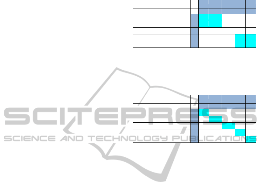
An initial modularity matrix (Table 11) was
obtained by straightforward linearity considerations:
eliminating empty and identical rows; an empty
column, “Electronic Lab Notebook”, was deleted. A
column was assigned to a next-level structor Data-
Discovery (DataDis) as it neatly fits the SearchData
functional. The scattered non-zero elements are
typical of initial matrices in this kind of analysis.
ICSOFT 2012 - 7th International Conference on Software Paradigm Trends
98
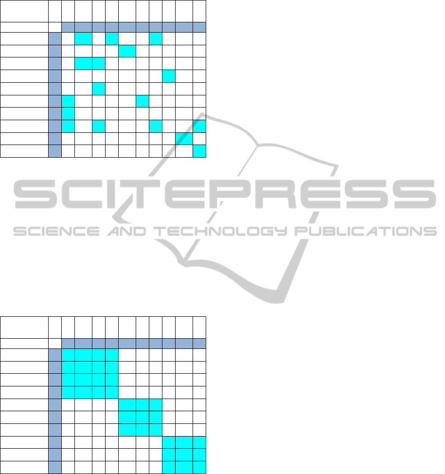
Table 11: NEESgrid initial Modularity Matrix.
Structors
chef
Data
Rp
Data
Vu
Data
Str
Data
Dis
Tele
pre
Data
Ac
Hyb
Exp
Sim
Rep
Grid
Infr
Functionals
1
2
3
4
5
6
7
8
9
10
Collect_Data
1
1
1
1
Search_Data
2
1
Manage_Data
3
1
1
HybridExper
4
1
Data_View
5
1
Sync_Collab
6
1
1
Async_Collab
7
1
Other_Collab
8
1
1
1
1
SimulCodes
9
1
HighPerfComp
10
1
Pure algebraic row/column reorder, without
semantic concerns, brings about the almost block-
diagonal Matrix (in Table 12). Its modules –
diagonal blocks – are:
Data manipulation – collect, search,
manage, view – the upper-left block;
Collaboration tools – synchronous, async,
other – the middle block;
Infrastructure – grid, codes – the lower-
right block.
Table 12: NEESgrid Bordered Linear-Reducible
Modularity Matrix.
Structors
Data
Str
Data
Dis
Data
Rp
Data
Vu
Data
Ac
Tele
pre
chef
Grid
Infr
Sim
Rep
Hybr
Exp
Functionals
4
5
2
3
7
6
1
10
9
8
Collect_Data
1
1
1
1
Search_Data
2
1
Manage_Data
3
1
1
Data_View
5
1
Other_Collab
8
1
1
1
1
Sync_Collab
6
1
1
Async_Collab
7
1
HighPerfComp
10
1
SimulCodes
9
1
HybridExper
4
1
Module interpretation is hinted by the respective
functional names – Data and Collab.
Outliers appear in the rows with maximal value
RowOffDiag=6, Collect_Data and Other_Collab.
The latter prefix "Other" hints at mixed functionals
to be decoupled.
This case study shows that: a- algebraic
reordering, without prior semantic knowledge,
obtains plausible modules; b- outliers are amenable
to interpretation, in particular matching project notes
(e.g. the row 8, column 10 outlier, marked "not
within the project scope” in project documents).
The significant result, common to large case
studies, is that there are few outliers, and all of them
are in columns/rows adjacent to the Linear Model
blocks. This is what we call bordered Linear-
Reducible.
4 DISCUSSION
4.1 Main Contribution: Linear
Software Models
This paper’s main contribution is the Linear
Software Models, as theoretical standards against
which to compare real software systems. The models
stand upon well-established linear algebra, as a
broad basis for a solid theory of composition –
beyond current principles and practices.
One can assert, from the Modularity Matrix
properties of a system, which structors are
independent and which functionals are
independently composable. One can then infer
which design improvements are desirable.
This view is very different from design models,
such as UML, whose purpose is not to serve as
theoretical standards. Design models freely evolve
with design and system development. Design models
have indefinite modifiability to adapt to any system,
in response to tests of system compliance to design.
4.2 Related Work
Matrices have been used to deal with modularity. A
prominent example is DSM (Design Structure
Matrix) proposed by Steward (Steward, 1981),
developed by Eppinger and collaborators e.g. (Sosa,
et al. 2005), (Sosa, et al. 2007)) and part of the
“Design Rules” approach by Baldwin and Clark –
see e.g. (Baldwin, Clark, 2000) and also (Cai,
Sullivan, 2006), (Sethi, et al. 2009). DSM and other
matrices, such as Kusiak and Huang’s (Kusiak,
Huang, 1997) hardware modularity matrix, are
meant to be evolving design models.
Linearity is the outstanding feature of our
standard models, not found in DSM. Essential
distinctions of Linear Software Models from DSM
are:
Theoretical Standards vs. Design Models –
our models’ goal is to serve as system
standards and ultimately may lead to
automatic software composition, as
Linear Software Models for Well-composed Systems
99

opposed to DSM design models which
emphasize design process and
manufacturing.
Functionals vs. Structures-only – our
modularity matrices display structor to
functional links, while both DSM matrix
dimensions are labeled by the same
structures.
Baldwin and Clark explicitly state in footnote 2,
page 63 of their book (Baldwin, Clark, 2000)
that “it is difficult to base modularity on functions…
hence their definition of modularity is based on
relationships among structures, not functions”. See
(Ulrich, 1995) for a different view.
In practice, modularity matrices may be much
more compact than DSM. For instance, Parnas’
KWIC DSM (Cai, Sullivan, 2006) has 20
rows/columns instead of just 5 in our Modularity
Matrix.
Although diagonality has seldom been calculated
within modularity, formulas have appeared in other
contexts. Clemins in (Clemins, et al. 2002) used for
speaker identification, the Frobenius norm – the sum
of the squares – of all off-diagonal elements to
measure diagonality. Our offdiag definition is better
suited to modularity, as it directly reflects distance to
the diagonal, while the Frobenius norm just sums
Boolean elements.
An indirect coupling metric is “similarity
coefficients” (Hwang, Oh, 2003), comparing matrix
row pairs, over all columns. The similarity for each
column is: both 1 elements, both 0, or different.
These coefficients ignore distances from the
diagonal.
The Modularity Matrix has a superficial
similarity to a traceability table. But their purposes
are definitely different. Traceability tables are used
to trace code and tests to requirements, while our
functionals' essence is to obtain measures of linear
independence.
The module detection literature is plentiful.
Tools to improve legacy code use clustering to
partition graphs (Mitchell, Mancoridis, 2006),
metrics to increase cohesion (Kang, Bieman, 1999)
and slicing of FDGs – Functional Dependence
Graphs (Rodrigues, Barbosa, 2006), tools to detect
modularity violations (Wong, et al., 2011). Even
with a quantitative flavor, they clearly differ from
the Linear Software Models’ approach.
4.3 Future Work
A mathematical characterization of modularity
matrix outliers deserves further investigation. This
relates to the broader issue of determining block
sizes, after exclusion of outliers, and module
refactoring.
A practical issue is to systematically obtain a
broad class of simple patterns strictly obeying the
Linear-Reducible Model – like the Observer – as
advocated for software building blocks.
Efficiency issues concerning modularity matrix
generation and reordering (cf. Borndorfer, et al.
1998) for large scale systems will be investigated.
This work has found that small software systems
are strictly Linear-Reducible, and some large
software systems are bordered Linear-Reducible.
This poses a variety of open questions.
The larger systems shown to be bordered Linear-
Reducible were developed before the proposal of the
Linear Model. It is conceivable, but still unclear, that
in view of this model they could be modified in a
natural way to comply with the strict Linear-
Reducible model. Similarly, future large scale
systems developed with awareness of linearity, may
show that strictly Linear-Reducibility rather than
limited to certain systems, is indeed applicable to a
wide variety of software systems.
4.4 Conclusions
Software has been perceived as essentially different
from other engineering fields, due to software’s
intrinsic variability, reflected in the soft prefix. This
versatility is often seen as an advantage to be
preserved, even though software composition has
largely resisted theoretical formalization.
We have found that Linear Software Models can
be formulated, without giving up variability. Thus,
software systems of disparate size, function and
purpose, may have Linearity in common.
REFERENCES
Baldwin, C.Y., and Clark, K.B., 2000. Design Rules, Vol.
I. The Power of Modularity, MIT Press, Cambridge,
MA, USA.
Borndorfer, R., Ferreira, C.E., and Martin, A., 1998.
“Decomposing Matrices into Blocks”, SIAM J.
Optimization, Vol. 9, Issue 1, pp. 236-269.
Cai, Y., and Sullivan, K.J., September 2006. “Modularity
Analysis of Logical Design Models”, in Proc. 21
st
IEEE/ACM Int. Conf. On Automated Software Eng.
ASE’06, pp. 91-102, Tokyo, Japan.
Clemins, P. J., Ewalt, H. E., and Johnson, M.T., 2002.
“Time-Aligned SVD Analysis for Speaker
Identification”, in Proc. ICASSP02 IEEE Int. Conf.
ICSOFT 2012 - 7th International Conference on Software Paradigm Trends
100

Acoustics Speech and Signal Proc., Vol. 4, pp. IV-
4160.
Finholt, T.A., Horn, D., and Thome, S., 2004. “NEESgrid
Requirements Traceability Matrix”, Technical Report
NEESgrid-2003-13, School of Information, University
of Michigan, USA.
Gamma, E., Helm, R., Johnson, R., and Vlissides, J.,
1995. Design Patterns: Elements of Reusable Object-
Oriented Software, Addison-Wesley, Boston, MA,
USA.
Hwang, H., and Oh, Y.H., 2003. “Another similarity
coefficient for the p-median model in group
technology”, Int. J. Manufacturing Tech. &
Management Vol. 5, pp. 38-245.
Kang, B-K., and Bieman, J.M., 1999. “A Quantitative
Framework for Software Restructuring”, J. Softw.
Maint. Research & Practice, Vol. 11, Issue 4, pp. 245-
284.
Kaufman, C., Perlman, R., and Speciner, M., 1997.
Network Security – Private Communication in a
Public World, Prentice-Hall, Englewood Cliffs, NJ,
USA.
Kusiak, A., and Huang, C-C., 1997. “Design of Modular
Digital Circuits for Testability”, IEEE Trans.
Components, Packaging and Manufacturing
Technology – Part C., Vol. 20, pp. 48-57 (1).
Martin, R. C., 2003. Agile Software Development:
Principles, Patterns and Practices, Prentice Hall,
Upper Saddle River, NJ.
Mitchell, B.S., and Mancoridis, S., 2006. “On the
Automatic Modularization of Software Systems Using
the Bunch Tool”, IEEE Trans. Software Engineering,
Vol. 32, pp. 193-208, (3).
Parnas, D.L., 1972. “On the Criteria to be Used in
Decomposing Systems into Modules”, Comm. ACM,
Vol. 15, pp. 1053-1058.
Riehle, D., 1996. “Describing and Composing Patterns
Using Role Diagrams”, in K-U. Mutzel & H-P. Frei.
(eds.) Proc. Ubilab Conf., Universitatsverlag
Konstanz, pp. 137-152.
Rodrigues, N.F., and Barbosa, L.S., 2006. "Component
Identification through program slicing", Electronic
Notes in Theoretical Computer Science, Vol. 160, pp.
291-304, Proc. Int. Workshop Formal Aspects of
Component Software (FACS 2005).
Rowland, T., and Weisstein, E.W., 2006. "Block Diagonal
Matrix." from MathWorld, http://
mathworld.wolfram.com/BlockDiagonalMatrix.html.
Sethi, K., Cai, Y., Wong, S., Garcia, A., and Sant’Anna,
C., 2009. “From Retrospect to Prospect: Assessing
Modularity and Stability from Software Architecture”,
in Proc. European Conf. on Software Architecture,
WICSA/ECSA, pp. 269-272.
Sosa, M.E., Agrawal, A., Eppinger, S.D., and Rowles,
C.M., September 2005. “A Network Approach to
Define Modularity of Product Components”, in Proc.
IDETC/CIE ASME International Design Engineering
Technical Conf. & Computers and Information in
Engineering Conf., Long Beach, CA, USA, pp. 1-12.
Sosa, M.E., Eppinger, S.D., and Rowles, C.M., 2007. “A
Network Approach to Define Modularity of
Components in Complex Products”, ASME Journal of
Mechanical Design, 129, 1118.
Steward, D., 1981. “The Design Structure System: A
Method for Managing the Design of Complex
Systems”, IEEE Trans. Eng. Manag., EM-29 (3), pp.
71-74.
Ulrich, K.T., 1995. “The Role of Product Architecture in
the Manufacturing Firm”, Res. Policy, 24, pp. 419-
440.
Wong, S., Cai, Y., Kim, M, and Dalton, M., 2011.
“Detecting Software Modularity Violations”, in Proc.
33
rd
Int. Conf. Software Engineering, pp. 411-420.
Linear Software Models for Well-composed Systems
101
