
Continue or Stop Reading? Modeling Decisions
in Information Search
Francisco L´opez-Orozco
1
, Anne Gu´erin-Dugu´e
2
and Benoˆıt Lemaire
1
1
LPNC, University of Grenoble, 38040 Grenoble Cedex 9, France
2
Gipsa-lab, University of Grenoble, 38042 Grenoble Cedex, France
Abstract. This paper presents a cognitive computational model of the way peo-
ple read a paragraph with the task of quickly deciding whether it is better related
to a given goal than another paragraph processed previously. In particular, the
model attempts to predict the time at which participants would decide to stop
reading the current paragraph because they have enough information to make
their decision. We proposed a two-variable linear threshold to account for that
decision, based on the rank of the fixation and the difference of semantic similar-
ities between each paragraph and the goal. Our model performance is compared
to the eye tracking data of 22 participants.
1 Introduction
Knowing what web users are doing while they search for information is crucial. Several
cognitive models have been proposed to account for some of the processes involved
in this activity. Pirolli & Fu [8] proposed a model of navigation. Brumby & Howes
[2] describes how people process information partially in order to select links related
to an information goal. Chanceaux et al. [3] show how visual, semantic and memory
processes interact in search tasks.
Information search can be made on any kind of documents, but we are here inter-
ested in textual documents, composed of several paragraphs.
Information search is different from pure reading because people have a goal in
mind while processing the document. They have to constantly keep in memory this
additional information. If the task is only to decide if the current paragraph is related or
not to the goal, that paragraph and the goal are the only pieces of information involved.
However, in everyday life, people are often concerned with deciding whether the current
paragraphis more interesting or not than another one that has been processed previously.
For instance, you are looking in a cookbook for a nice French recipe, you already found
one but you want to find a better one. In that case, at least three pieces of information
have to be together managed in order to make a correct decision: the current paragraph,
the goal and a previous paragraph.
This paper attempts to model that particular decision making. It focuses on a be-
havior that is specific to information search, which is stopping processing a paragraph
before it is completely read.
López-Orozco F., Guérin-Dugué A. and Lemaire B..
Continue or Stop Reading? Modeling Decisions in Information Search.
DOI: 10.5220/0004099900960105
In Proceedings of the 9th International Workshop on Natural Language Processing and Cognitive Science (NLPCS-2012), pages 96-105
ISBN: 978-989-8565-16-7
Copyright
c
2012 SCITEPRESS (Science and Technology Publications, Lda.)
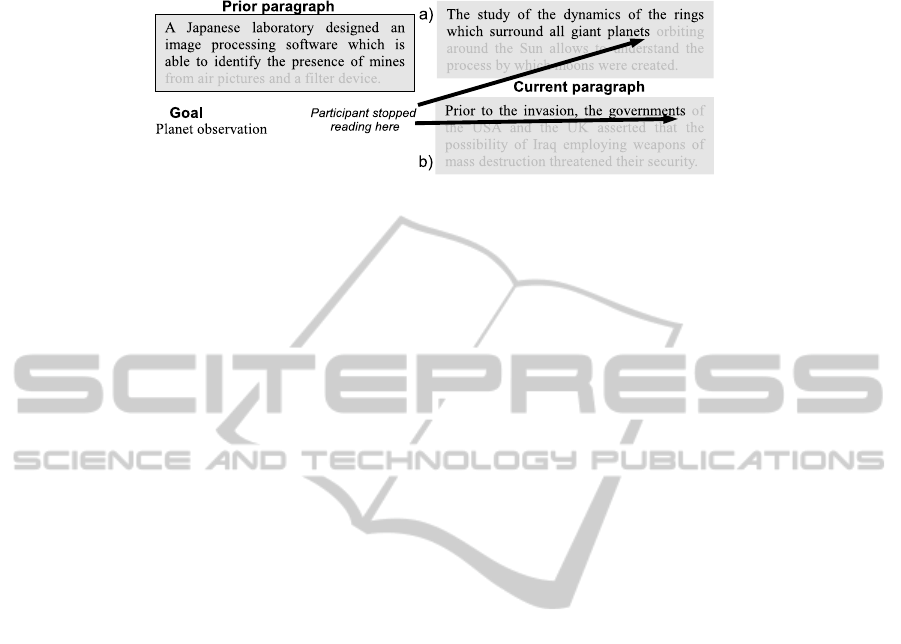
Fig.1. Illustration of the 3 input data of the model: prior paragraph, goal, current paragraph. Prior
paragraph has been processed partially. Current paragraph is abandoned before its end because
enough information has been gathered and maybe due to a) a high-relatedness to the goal b) a
low-relatedness to the goal.
This particular problem has been studied by Lee and Corlett [6]: participants were
provided with a topic and a text, presented one word every second, and were asked to
decide as quickly as possible if the text is about the given topic. However, we aim at
studying a normal reading situation instead of presenting one word at a time. We will
therefore rely on an eyetracker to identify the words processed. Figure 1 illustrates the
situation we aim at modeling.
2 Experiment
In order to create and study a model, we designed an experiment to gather some data.
This experiment was intended to emphasize the decision to stop reading a paragraph
while two other pieces of information are stored in memory: another paragraph and
the search goal. A set of 20 goals was created. Each one is expressed by a few words
(e.g. mountain tourism). For each goal, 7 paragraphs were created (mean=30.1 words,
σ=2.9), 2 of them being highly related to the goal, 2 of them being moderately related,
and 3 of them being unrelated. We used Latent Semantic Analysis (LSA) (Landauer
et al., [5]) to control the relatedness of a paragraph to the goal. Basically, LSA takes a
large corpus as input and yields a high-dimensional vector representation for each word.
It is based on a singular value decomposition of a word x paragraph occurrence matrix,
where words occurring in similar contexts are represented by similar vectors. Such a
vector formalism is very convenient to give a representation to sentences that were not
in the corpus: the meaning of a new sentence is represented as a linear combination of
its word vectors. Therefore, any sequence of words can be given a representation. The
semantic similarity between two sequences of words (such as a goal and a paragraph)
can be computed using the cosine function. The higher the cosine value, the more sim-
ilar the two sequences of words. We trained LSA on a 24 million word general French
corpus.
The experiment is composed of 20 trials, each one corresponding to a goal, in ran-
dom order. In each trial, 2 paragraphs are presented together to the participant, as well
as the goal (Fig. 2). The participant should select which paragraph is best related to the
goal, by typing one key. The chosen paragraph is kept and the other is replaced by a
new one. The participant should again select the most related to the goal. Then another
97

Fig.2. Example of material and scanpath.
paragraph replaces the one that was not selected and so on. This procedure is repeated
until all 7 paragraphs of the current goal were displayed. Participants rated their confi-
dence in their selection. Each participant was therefore exposed to 20*6=120 pairs of
paragraphs, and selected for each pair the paragraph which is most related to the goal.
22 participants participated in the experiment. Eye movements were recorded using a
SR Research EyeLink II eye tracker. From these coordinates, saccades and fixations
were determined, leading to an experimental scanpath, as shown in Fig. 2. The stimuli
pages were generated with a software that stored the precise coordinates of each word
on the screen. We wrote our experiment in Matlab, using the Psychophysics Toolbox
(Brainard, [1]). Before trying to mimic eye movements, we had to predict which words
were actually processed by participants in each fixation. It is known that the area from
which information can be extracted during a single fixation extends from about 3-4
characters to the left of fixation to 14-15 characters to the right of fixation (Rayner,
[10]). This area is asymmetric to the right and corresponds to the global perceptual
span. Therefore, more than one word may be processed for a given fixation. In order
to determine which ones were processed for each fixation, we used a window, sized
according to Rayner [10]. He showed that the area from which a word can be identified
extends to no more than 4 characters to the left and no more than 7-8 characters to the
right of fixation and corresponds to the word identification span. Moreover, Pollatsek
et al [9] show that even if information of the next line is processed during a reading
task, participants are not capable of getting some semantic information. Therefore, the
size of our window is 4 x 1 characters to the left plus 8x1 characters to the right of the
fixation point. Since the initial fixations in the beginning part of a word facilitate its
recognition more than initial fixations toward the end of the word (Farid & Grainger,
[4]), we considered that a word is processed if at least the first third of it or the last
two-thirds is inside the window.
3 Modeling
The model should be able to predict the way a paragraph is processed, given a previous
paragraph and a goal. For example, given the left paragraph of Fig. 2 and the goal,
the model should be able to predict the way an average user would process the right
paragraph (in this case the paragraph is processed partially).
98

Our method is therefore to consider the experimental scanpaths and for each partic-
ipant’s fixation to predict whether the paragraph would be abandoned or not. A very
good model would predict an abandon at the same time the participant stopped reading.
A bad model would abandon too early or too late.
Paragraphs can be examined several times by participants during a trial, but we
restricted our analysis to first visits of the current paragraph. It is also worth noting
that the previous paragraph is not necessary on the same stimuli page as the current
paragraph. It could have been seen on the previous stimuli page. That is for instance the
case of the left paragraph of Fig. 2 which has been processed with another paragraph in
mind, seen on the previous stimuli page.
3.1 Modeling Semantic Judgments
Such a decision making model on paragraphs needs to be based on a model of semantic
memory that would be able to mimic human judgments of semantic associations. We
used LSA to dynamically compute the semantic similarities between the goal and each
set of words that are supposed to have been fixated.
We assumed a linear exploration of words, although we know that this is not exactly
the case in information search (Chanceaux et al., [3]).
3.2 Effect of the Prior Paragraph
The relatedness of the prior paragraph to the goal may play a role in the way the current
paragraph is processed. We suspected that if the prior paragraph is not related to the
goal, the current paragraph would be processed just to check whether it is relevant
or not. The prior paragraph would not play a role in that case. However, if the prior
paragraph is related to the goal, then the current paragraph may be processed with the
idea of comparing it to the previous one.
We therefore analyzed two extreme cases: the words fixated in the prior paragraph
are strongly related to the goal or they are not related at all to the goal. We used two
thresholds of cosine similarity for that, which were set to 0.05 and 0.25. Paragraphs
whose semantic similarity with the goal falls in between were not considered. The first
case is called C—S (read the Current knowing that the previous one is Strong) and
the second one is called C—W (Current — Previous=Weak). We also analyzed cases
when no prior paragraph exists, called C—0 (Current — Nothing). Basic statistics show
that in terms of number of fixations, fixation duration and the shape of the scanpath,
C—W=C—0 and both are significantly different from C—S. It means that reading a
paragraph while the other one is not related to the goal is similar to reading the very
first paragraph, without information about a prior paragraph.
Therefore we will only consider the case C—S in this paper: reading a paragraph
with another one in mind which is highly related to the goal.
3.3 Modeling the Decision
Two Variables Involved. We first looked for the variables which could play a role in
the decision to stop reading a paragraph. Such a decision is made when the difference
99
(a) (b)
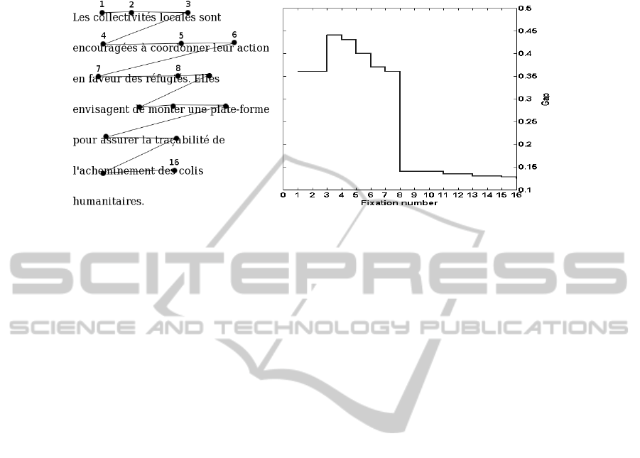
Fig.3. a) Example of scanpath in the C—S condition. b) Its Gap evolution.
between the current (cp) and the previous paragraph (pp) is large enough to know
for sure which one is the best. If they are too close to each other, no decision can be
made and reading is pursued. The association to the goal g is obviously involved in
that perception of a difference between the two paragraphs. Therefore, we defined a
variable called Gap = |sim(words of pp, g) −sim(words of cp, g)| in which sim is the
LSA cosine between the two vectors.
Gap changes constantly while a paragraph is processed since it depends on the
words actually processed. When the two paragraphs are equally similar to the goal,
that variable is zero. When one paragraph is much more associated to the goal than
the other one, that variable has a high value. It can be easily calculated dynamically,
after each word of the current paragraph has been processed. Consider for example Fig.
3(a). Suppose that a prior paragraph has already been visited (paragraph and goal are
not shown) and the sequence of words processed so far has led to a similarity sim
1
with the goal “associations humanitaires” of 0.62. In the first two fixations on the
current paragraph, only the word “collectivit
´
es” is supposed to have been processed
according to our window-based prediction. Therefore in both cases Gap = |sim
1
−
sim(“collectivit
´
es”,“associations humanitaires”)| = 0.62 - 0.26 = 0.36.
During fixation 3, two extra words were processed leading to a new value of Gap =
|sim
1
−sim(“collectivit
´
es locales sont”,“associations humanitaires”)| = 0.44. In fixa-
tion 4, Gap = |sim
1
−sim(“collectivit
´
es locales sont encourag
´
ees
`
a”,
“associations humanitaires”)| = 0.43. In fixation number 5, Gap = |sim
1
−sim(“collec
tivit
´
es locales sont encourag
´
ees
`
a coordonner leur”, “associations humanitaires”)— =
0.40. In fixation 8, the Gap value dropped to 0.14 because of the word “r
´
efugi
´
es” which
makes the LSA vector much more similar to the goal vector. Figure 3(b) shows the evo-
lution of the Gap value along the fixations in the scanpath. This example illustrates that
a high value of Gap may not directly induce the decision, in particular if it appears
too early in the scanpath. We assume that the decision also depends on the number of
words processed so far in the current paragraph. The more words processed, the higher
the confidence in the perception of the difference between paragraphs. If only two or
three words have been processed, it is less likely that Gap is accurate. Therefore, we
100

(a) (b)
Fig.4. a) Empirical “no-abandon” distribution ˆp
GR
(g, r|Ab) and b) “abandon” distribution
ˆp
GR
(g, r|Ab) in the Gap×Rank space.
assume that there should be a relationship between Gap and the number of words pro-
cessed. The second variable is then Rank = number of words processed so far.
Abandon and No-abandon Distributions. In order to study how the decision depends
on these two variables, we computed two distributions in the Gap ×Rank space of
participant data: the distribution of the no-abandon cases and the distribution of the
abandon cases. The goal is to learn the frontier between both cases in order to be able
to predict if a sequence of words already processed is likely to lead to the abandon or
the pursuance of the reading task. This work was done on two thirds of the data, in
order to leave one third to test the model. Each participant fixation was associated to a
point in the Gap×Rank space. Rank is a discrete measure between 1 and the maximum
number of fixations in the data (93 in our case). Gap has been computed according to
the previousformula,taking into account the words already processed in each paragraph
as well as the goal and discretized into one of 100 bins, from 0 to 1.
The no-abandon distribution was computed by simply counting the number of fixa-
tions that did not lead to an abandon for each cell of the Gap×Rank grid. It concerns
all fixations except the last one of each scanpath.
The abandon distribution was built from all very last fixations of all scanpaths, in-
cluding also subsequent ranks. For example, if a given participant on a given stimulus
made 13 fixations, the first 12 were counted in the no-abandon distribution and the 13th
was counted in the abandon distribution. All virtual fixations from 14 to 93, with the
same gap value as the 13th were also counted in the abandon distribution, because if the
participant stopped reading at fixation 13, he would have also stopped at fixation 14, 15,
etc. The frontier between these two behaviors (continue or stop reading) is a curve in the
Gap×Rank space. Depending on the location of any observation (g,r) above or under
the curve, the reader’s behavior can be predicted. To find this frontier, a methodology
based on a Bayesian classifier is used. Let us consider a classification problem with two
classes: Abandon (Ab) and No-abandon (Ab). Given the posterior probabilities, which is
the class of a two-dimensional observation (g,r) in the Gap×Rank space? The decision
rule is then:
101

P(Ab|g, r)
Ab
≷
Ab
P(Ab|g, r),
with P(Ab|g, r) =
P(Ab)×p
GR
(g,r|Ab)
p
GR
(g,r)
, and P(Ab|g, r) =
P(Ab)×p
GR
(g,r|Ab)
p
GR
(g,r)
. Figures 4(a) and
4(b) represent the two empirical class-conditional probability density functions respec-
tively ˆp
GR
(g, r|Ab) and ˆp
GR
(g, r|Ab). We adopt a statistical parametric approach. By
this way, data will be regularized since they are obviously affected by the noise inher-
ent to acquisition and pre-processing.
In the next sections, the statistical model to estimate the density functions and the
prior probabilities are explained in order to use the Bayesian classifier:
P(Ab) × p
GR
(g, r|Ab)
Ab
≷
Ab
P(Ab) × p
GR
(g, r|Ab).
Parametric Model for the “No-abandon” Distribution. The class-conditional proba-
bility density function can be written as : p
GR
(g, r|Ab) = p
G|R
(g|R = r, Ab)×p
R
(r|Ab).
Figure 5 (top, left) shows the empirical marginal distribution ˆp
R
(r|Ab). As the Rank in-
creases, the probability of not abandoning the paragraph decreases. This evolution was
modeled with a sigmoid function ϕ(r) =
P
RMax
×
(
1+e
−αr
0
)
1+e
α(r−r
0
)
. There are actually only two
parameters to fit because the integral is 1.
Fig.5. Data and fitting of marginal distributions, mean and standard deviation for the “no-
abandon” and “abandon” distributions.
Concerning the probability density function p
G|R
(.), the natural model (Fig. 4(a))
is a Gaussian one whose parameters depend on the Rank value. The mean µ(r) and the
standard deviation σ(r) linearly decrease (Fig. 5, left column). The linear regressions
are only performed up to the Rank=40 since that ˆp
R
(r > 40|Ab) is close to zero and
there is no more enough data. Then we have:
p
G|R
(g|R = r, Ab) =
A(r)
√
2πσ(r)
e
−
(g−µ(r))
2
2σ(r)
2
, p
R
(r, Ab) = ϕ(r).
102

As the Gap value is between 0 and 1, A(r) is a normalization function to ensure that
p
G|R
(g|R= r, Ab) is a probabilitydensity function: A(r) = F
µ,σ
(1)−F
µ,σ
(0), with F
µ,σ
(.)
being the repartition function of a Gaussian distribution with a mean µ and a standard
deviation σ. We then obtained six independent parameters to model the complete “no-
abandon” joint distribution (offset and slope for the sigmoid, and the two linear func-
tions).
Parametric Model for the “Abandon” Distribution. Following a similar approach
the class-conditional pdf is written as : p
GR
(g, r|Ab) = p
G|R
(g|R = r, Ab) × p
R
(r|Ab).
The marginal pdf ˆp
R
(r|Ab) was modeled with another sigmoid function ϕ
′
(r) (Fig. 5,
top right). But here, it is an increasing function. At rank 0, there is no abandon and at
the maximal Rank value, all scanpaths have shown an abandon. The conditional dis-
tribution ˆp
G|R
(g|R = r, Ab) is a Gaussian distribution with a mean µ
′
(r) and a standard
deviation σ
′
(r). The mean µ
′
(r) exponentially decreases while the standard deviation
σ
′
(r) exponentially increases (Fig. 5, right column). Equations of the pdf are the same
as the previous case, but with a different set of functions {ϕ
′
(r),µ
′
(r),σ
′
(r)} which gives
us seven parameters (2 for the ϕ
′
(r), 3 for µ
′
(r) and 2 for σ
′
(r)):
p
G|R
(g|R = r, Ab) =
A
′
(r)
√
2πσ
′
(r)
e
−
(g−µ
′
(r))
2
2σ
′
(r)
2
, p
R
(r, Ab) = ϕ
′
(r).
Modeling the Decision as the Function of Rank and Gap. As these two class-conditio-
nal probabilities were modeled, for each (Rank, Gap) values, the problem is to decide
if there is enough information to stop reading (“abandon” class), or to continue read-
ing (“no abandon” class). This binary problem is solved thanks to the Bayesian classi-
fier. To find this decision rule, we have now to estimate the prior probabilities such as:
P(Ab) + P(Ab) = 1. P(Ab) or P(Ab) is another parameter to learn from the data. The
total number of learning parameters is then 14 (6+7+1). The decision rule is then:
P(Ab) × p
G|R
(g|R = r, Ab) × p
R
(r|Ab)
Ab
≷
Ab
P(Ab) × p
G|R
(g|R = r, Ab)× p
R
(r|Ab).
4 Model Learning
Figure 6 shows the two posterior probabilities P(Ab|g, r) and P(Ab|g, r) after learn-
ing in order to represent the decision frontier between the two classes. The two prior
probabilities are P(Ab) = 0.84 and P(Ab) = 0.16. As Fig. 6 shows, the intersection is
oblique which is what was expected, from a cognitive point of view. Rank and Gap are
dependent on each other: at the beginning of processing the paragraph (low values of
the Rank), there should be a high difference between the two paragraphs to make the
decision. However, after more fixations have been made, that difference could be lower
to decide to abandon the paragraph.
For instance, at rank 10, a Gap of .86 is necessary to stop reading, whereas at rank
15, a value of .42 is enough. The frontier is rather linear and can be approximated by
the following equation in the Gap×Rank space:
Gap
0
= −0.090 ×Rank + 1.768.
103
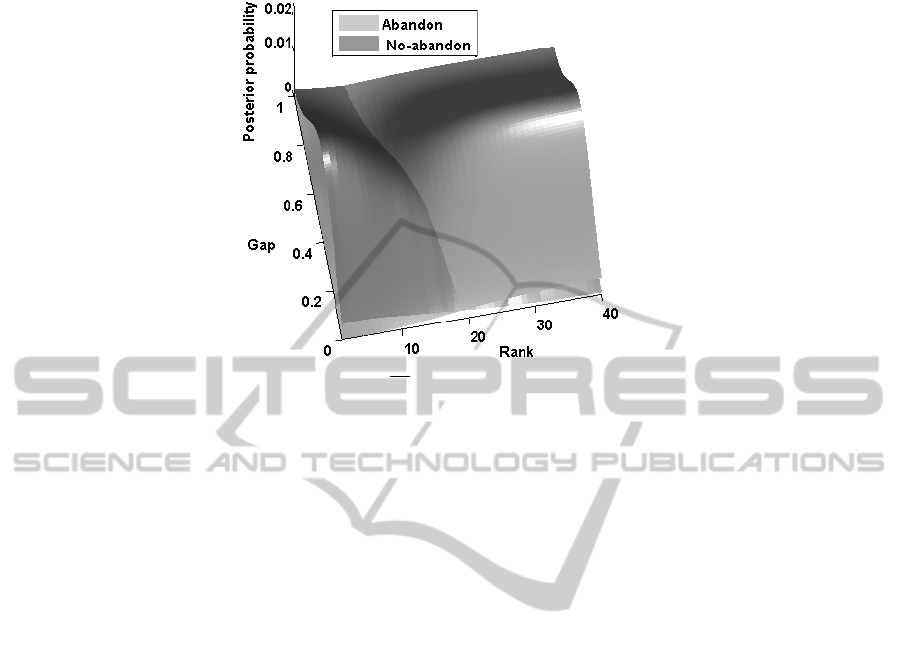
Fig.6. The posterior probabilities P(Ab|g, r) and P(Ab|g, r) in the Gap×Rank space.
That equation was included in the computational model. That model constantly com-
putes the Gap value while it is moving forward in the text, increasing the Rank value.
As soon as the current Gap value is greater than Gap
0
, the decision is to stop reading
the paragraph.
In order to test the model, we ran it on the remaining one third of the data. For each
fixation in this testing set, the model decides either to leave or not to leave the para-
graph. If the model did not leave at the time the participant stopped reading, simulation
is pursued with the next rank and with the same value of the gap, and so on until the
decision is made. The average difference between the ranks at which model and par-
ticipant stopped reading was computed. We got a value of 6.58 (SE=0.29). To assess
the significance of that value, we built a random model which stops reading after each
fixation with probability p. The smallest average difference between participants’ and
model’s ranks of abandoning was 11.47 (SE=0.45) and was obtained for p = 0.20. Our
model therefore appears to be much better than the best random model.
5 Conclusions
We presented a model which predicts the sequence of words that are likely to be fixated
before a paragraph is abandoned given a search goal. Two variables seem to play a
role: the rank of the fixation and the difference of semantic similarities between each
paragraph and the search goal. We proposed a simple linear threshold to account for
that decision. Our model will be improved in future work. In particular, we aim at
considering a non linear way of scanning the paragraph, using another model of eye
movements (Lemaire et al., [7]). We also plan to tackle more realistic stimuli as well as
extending that approach to consider other decisions involved in Web search tasks.
104

References
1. Brainard, D. H.: The Psychophysics Toolbox, Spatial Vision 10(1997) 433–436.
2. Brumby, D. P., Howes, A.: Good enough but I’ll just check: Web-paged search as attentional
refocusing. In Proc of the 6th ICCM Conference (2004) 46–51.
3. Chanceaux, M., Gu´erin-Dugu´e, A., Lemaire, B., Baccino, T.: A model to simulate Web users’
eye movements. In Proc of the 12th INTERACT Conference, LNCS 5726, Berlin: Springer
Verlag, (2009) 288–300.
4. Farid, M., Grainger, J. How initial fixation position influences word recognition: A compar-
ison of French and Arabic. Brain & Language, 53, (1996) 351–368.
5. Landauer, T., McNamara, D., Dennis, S., Kintsch, W.: Handbook of Latent Semantic Analy-
sis. Lawrence Erlbaum Associates, (2007).
6. Lee, M. D., Corlett, E. Y. Sequential sampling models of human text classification. Cognitive
Science, 27(2), (2003) 159–193.
7. Lemaire, B., Gu´erin-Dugu´e, A., Baccino, T., Chanceaux, M., Pasqualotti, L.: A cognitive
computational model of eye movements investigating visual strategies on textual material.
In L. Carlson, C. Hlscher and T. Shipley (Eds.) Proc of the Annual Meeting of the Cognitive
Science Society, (2011) 1146–1151.
8. Pirolli, P., & Fu, W. SNIF-ACT: a model of information foraging on the world wide web. In
P. Brusilovsky, A. Corbett, & F. de Rosis (Eds.), 9th ICUM (2003) 45–54.
9. Pollatsek, A., Raney, G. E., LaGasse, L., & Rayner, K.: The use of information below fixation
in reading and in visual search. Can J Psychol 47, (1993) 179–200.
10. Rayner, K. Eye movements in reading and information processing: 20 years of research.
Psychological Bulletin 124(3), (1998) 372–422.
105
