
Diffusion Ensemble Classifiers
Alon Schclar
1
, Lior Rokach
2
and Amir Amit
3
1
School of Computer Science, Academic College of Tel Aviv-Yaffo, P.O.B 8401, Tel Aviv 61083, Israel
2
Department of Information Systems Engineering, Ben-Gurion University of the Negev,
P.O.B 653, Beer-Sheva 84105, Israel
3
The Efi Arazi School of Computer Science, Interdisciplinary Center (IDC) Herzliya, P.O.B 167, Herzliya 46150, Israel
Keywords:
Ensemble Classifiers, Dimensionality Reduction, Out-of-Sample Extension, Diffusion Maps, Nystr¨om
Extension.
Abstract:
We present a novel approach for the construction of ensemble classifiers based on the Diffusion Maps (DM)
dimensionality reduction algorithm. The DM algorithm embeds data into a low-dimensional space according
to the connectivity between every pair of points in the ambient space. The ensemble members are trained
based on dimension-reduced versions of the training set. These versions are obtained by applying the DM
algorithm to the original training set using different values of the input parameter. In order to classify a test
sample, it is firstembedded into the dimension reduced space of each individual classifier by using the Nystr¨om
out-of-sample extension algorithm. Each ensemble member is then applied to the embedded sample and the
classification is obtained according to a voting scheme. A comparison is made with the base classifier which
does not incorporate dimensionality reduction. The results obtained by the proposed algorithms improve on
average the results obtained by the non-ensemble classifier.
1 INTRODUCTION
Classifiers are predictive models which label data
based on a training dataset T whose labels are known
a-priory. A classifier is constructed by applying an
induction algorithm, or inducer, to T - a process that
is commonly known as training. Classifiers differ
by the induction algorithms and training sets that are
used for their construction. Common induction algo-
rithms include nearest neighbors (NN), decision trees
(CART (Breiman et al., 1993), C4.5 (Quinlan, 1993)),
Support Vector Machines (SVM) (Vapnik, 1999) and
Artificial Neural Networks - to name a few. Since
every inducer has its advantages and weaknesses,
methodologies have been developed to enhance their
performance. Ensemble classifiers are one of the most
common ways to achieve that.
The need for dimensionality reduction techniques
emerged in order to alleviate the so called curse of di-
mensionality - the fact that the complexity of many al-
gorithms grows exponentially with the increase of the
input data dimensionality (Jimenez and Landgrebe,
1998). In many cases a high-dimensional dataset lies
approximately on a low-dimensional manifold in the
ambient space. Dimensionality reduction methods
embed datasets into a low-dimensional space while
preserving as much possible the information that is
conveyed by the dataset. The low-dimensional rep-
resentation is referred to as the embedding of the
dataset. Since the information is inherent in the ge-
ometrical structure of the dataset (e.g. clusters), a
good embedding distorts the structure as little as pos-
sible while representing the dataset using a number of
features that is substantially lower than the dimension
of the original ambient space. Furthermore, an effec-
tive dimensionality reduction algorithm also removes
noisy features and inter-feature correlations.
1.1 Ensembles of Classifiers
Ensembles of classifiers (Kuncheva, 2004) mimic the
human nature to seek advice from several people be-
fore making a decision where the underlying assump-
tion is that combining the opinions will produce a de-
cision that is better than each individual opinion. Sev-
eral classifiers (ensemble members) are constructed
and their outputs are combined - usually by voting or
an averaged weighting scheme - to yield the final clas-
sification (Polikar, 2006; Opitz and Maclin, 1999).
In order for this approach to be effective, two crite-
443
Schclar A., Rokach L. and Amit A..
Diffusion Ensemble Classifiers.
DOI: 10.5220/0004102804430450
In Proceedings of the 4th International Joint Conference on Computational Intelligence (NCTA-2012), pages 443-450
ISBN: 978-989-8565-33-4
Copyright
c
2012 SCITEPRESS (Science and Technology Publications, Lda.)

ria must be met: accuracy and diversity (Kuncheva,
2004). Accuracy requires each individual classifier to
be as accurate as possible i.e. individually minimize
the generalization error. Diversity requires minimiz-
ing the correlation among the generalization errors of
the classifiers. These criteria are contradictory since
optimal accuracy achieves a minimum and unique er-
ror which contradicts the requirement of diversity.
Complete diversity, on the other hand, corresponds
to random classification which usually achieves the
worst accuracy. Consequently, individual classifiers
that produce results which are moderately better than
random classification are suitable as ensemble mem-
bers.
In this paper we focus on ensemble classifiers
that use a single induction algorithm, for example
the Na¨ıve Bayes inducer. This ensemble construc-
tion approach achieves its diversity by manipulating
the training set. A well known way to achieve diver-
sity is by bootstrap aggregation (Bagging) (Breiman,
1996). Several training sets are constructed by apply-
ing bootstrap sampling (each sample may be drawn
more than once) to the original training set. Each
training set is used to construct a different classi-
fier where the repetitions fortify different training in-
stances. This method is simple yet effective and has
been successfully applied to a variety of problems
such as spam detection (Yang et al., 2006), analysis
of gene expressions (Valentini et al., 2003) and user
identification (Feher et al., 2012).
The award winning Adaptive Boosting (Ad-
aBoost) (Freund and Schapire, 1996) algorithm and
its subsequent versions e.g. (Drucker, 1997) and
(Solomatine and Shrestha, 2004) provide a different
approach for the construction of ensemble classifiers
based on a single induction algorithm. This approach
iteratively assigns weights to each training sample
where the weights of the samples that are misclassi-
fied are increased according to a global error coeffi-
cient. The final classification combines the logarithm
of the weights to yield the ensemble’s classification.
Successful applications of the ensemble method-
ology can be found in many fields such as recom-
mender systems (Schclar et al., 2009), classification
(Schclar and Rokach, 2009), finance (Leigh et al.,
2002), manufacturing (Rokach, 2008) and medicine
(Mangiameli et al., 2004), to name a few.
1.2 Dimensionality Reduction
The dimensionality reduction problem can be for-
mally described as follows. Let
Γ = {x
i
}
N
i=1
(1)
be the original high-dimensional dataset given as a set
of column vectors where x
i
∈ R
n
, n is the dimension
of the ambient space and N is the size of the dataset.
All dimensionality reduction methods embed the vec-
tors into a lower dimensional space R
q
where q ≪ n.
Their output is a set of column vectors in the lower
dimensional space
e
Γ = {ex
i
}
N
i=1
, ex
i
∈ R
q
(2)
where q is chosen such that it approximates the in-
trinsic dimensionality of Γ (Hein and Audibert, 2005;
Hegde et al., 2007). We refer to the vectors in the set
e
Γ as the embedding vectors.
Dimensionality techniques can be divided into
global and local methods. The former derive em-
beddings in which all points satisfy a given crite-
rion. Examples for global methods include: Principal
Component Analysis (PCA) (Hotelling, 1933), Ker-
nel PCA (KPCA) (Sch¨olkopf et al., 1998; Sch¨olkopf
and Smola, 2002), Multidimensional scaling (MDS)
(Kruskal, 1964; Cox and Cox, 1994), ISOMAP
(Tenenbaum et al., 2000), etc. Contrary to global
methods, local methods construct embeddings in
which only local neighborhoods are required to meet
a given criterion. The global description of the dataset
is derived by the aggregation of the local neighbor-
hoods. Common local methods include Local Linear
Embedding (LLE) (Roweis and Saul, 2000), Lapla-
cian Eigenmaps (Belkin and Niyogi, 2003), Hes-
sian Eigenmaps (Donoho and Grimes, 2003) and Dif-
fusion Maps (Coifman and Lafon, 2006a; Schclar,
2008) which is used in this paper and is described in
Section 3.
A key aspect of dimensionality reduction is how to
efficiently embed a new point into a given dimension-
reduced space. This is commonly referred to as out-
of-sample extension where the sample stands for the
original dataset whose dimensionality was reduced
and does not include the new point. An accurate em-
bedding of a new point requires the recalculation of
the entire embedding. This is impractical in many
cases, for example, when the time and space com-
plexity that are required for the dimensionality reduc-
tion is quadratic (or higher) in the size of the dataset.
An efficient out-of-sample extension algorithm em-
beds the new point without recalculating the entire
embedding - usually at the expense of the embedding
accuracy.
The Nystr¨om extension (Nystr¨om, 1928) algo-
rithm, which is used in this paper, embeds a new point
in linear time using the quadrature rule when the di-
mensionality reduction involves eigen-decomposition
of a kernel matrix. Algorithms such as Diffusion
Maps, Laplacian Eigenmaps, ISOMAP, LLE, etc. are
IJCCI2012-InternationalJointConferenceonComputationalIntelligence
444
Inducer
Parameter
values
1
Parameter
values
K
Original
Training
Set
Training
Set
1
Training
Set
K
Classifier
1
Classifier
K
The Ensemble
Diffusion
Maps
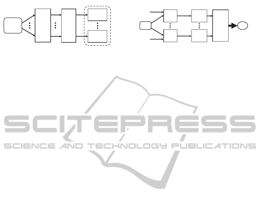
Figure 1: Ensemble training.
examples that fall into this category and, thus, the em-
beddings that they produce can be extended using the
Nystr¨om extension (Ham et al., 2004; Bengio et al.,
2004). A formal description of the Nystr¨om exten-
sion is given in the Sec. 4.
The main contribution of this paper is a novel
framework for the construction of ensemble classi-
fiers based on the Diffusion Maps dimensionality re-
duction algorithm coupled with the Nystr¨om out-of-
sample extension. The rest of this paper is orga-
nized as follows. In Section 2 we describe the pro-
posed approach. In Section 3 we describe the Diffu-
sion Maps dimensionality reduction algorithm. The
Nystr¨om out-of-sample extension algorithm is de-
scribed in Section 4. Experimental results are given
in Section 5. We conclude and describe future work
in Section 6.
2 DIFFUSION ENSEMBLE
CLASSIFIERS
The proposed approach achieves the diversity require-
ment of ensemble classifiers by applying the DM di-
mensionality reduction algorithm to a given training
set using different values for its input parameter. After
the training sets are produced by the DM dimension-
ality reduction algorithms, each set is used to train a
classifier to produce one of the ensemble members.
The training process is illustrated in Fig. 1.
Employing the DM dimensionality reduction to a
training set has the following advantages:
• It reduces noise and decorrelates the data.
• It reduces the computational complexity of the
classifier construction and consequently the com-
plexity of the classification.
• It can alleviate over-fitting by constructing com-
binations of the variables (Plastria et al., 2008).
These points meet the accuracy and diversity criteria
which are required to construct an effective ensemble
classifier and thus render dimensionality reduction a
technique which is tailored for the construction of en-
semble classifiers. Specifically, removing noise from
Voting
Out-of-
sample
Extension
Out-of-
sample
Extension
Classifier
1
Classifier
K
Class
Parameters
1
and
Training
Set
1
Test
Sample
Parameters
M
and
Training
Set
K
Embedded
Test Sample
1
Embedded
Test Sample
K
Figure 2: Classification process of a test sample.
the data contributes to the accuracy of the classifier
while diversity is obtained by the various dimension-
reduced versions of the data.
In order to classify test samples they are first em-
bedded into the low-dimensional space of each of
the training sets using the Nystr¨om out-of-sample ex-
tension. Next, each ensemble member is applied to
its corresponding embedded test sample and the pro-
duced results are processed by a voting scheme to de-
rive the result of the ensemble classifier. Specifically,
each classification is given as a vector containing the
probabilities of each possible label. These vectors are
aggregated and the ensemble classification is chosen
as the label with the largest probability. Figure 2 de-
picts the classification process of a test sample.
3 DIFFUSION MAPS
The Diffusion Maps (DM) (Coifman and Lafon,
2006a) algorithm embeds data into a low-dimensional
space where the geometry of the dataset is defined in
terms of the connectivity between every pair of points
in the ambient space. Namely, the similarity between
two points x and y is determined according to the
number of paths connecting x and y via points in the
dataset. This measure is robust to noise since it takes
into account all the paths connecting x and y. The
Euclidean distance between x and y in the dimension-
reduced space approximates their connectivity in the
ambient space.
Formally, let Γ be a set of points in R
n
as defined
in Eq. 1. A weighted undirected graph G(V,E), |V|=
N, |E| ≪ N
2
is constructed, where each vertex v ∈V
corresponds to a point in Γ. The weights of the edges
are chosen according to a weight function w
ε
(x,y)
which measures the similarities between every pair of
points where the parameter ε defines a local neighbor-
hood for each point. The weight function is defined by
a kernel function obeying the following properties:
Symmetry: ∀x
i
,x
j
∈Γ, w
ε
(x
i
,x
j
) = w
ε
(x
j
,x
i
)
Non-negativity: ∀x
i
,x
j
∈Γ, w
ε
(x
i
,x
j
) ≥ 0
Positive Semi-definite: for every real-
valued bounded function f defined on Γ,
DiffusionEnsembleClassifiers
445

∑
x
i
,x
j
∈Γ
w
ε
(x
i
,x
j
) f (x
i
) f (x
j
) ≥ 0.
Fast Decay: w
ε
(x
i
,x
j
) → 0 when
x
i
−x
j
≫ ε and
w
ε
(x
i
,x
j
) →1 when
x
i
−x
j
≪ε. This property
facilitates the representation of w
ε
by a sparse ma-
trix.
A common choice that meets these criteria is the
Gaussian kernel:
w
ε
(x
i
,x
j
) = e
−
k
x
i
−x
j
k
2
2ε
.
A weight matrix w
ε
is used to represent the
weights of the edges. Given a graph G, the Graph
Laplacian normalization (Chung, 1997) is applied to
the weight matrix w
ε
and the result is given by M:
M
i, j
, m(x,y) =
w
ε
(x,y)
d (x)
where d(x) =
∑
y∈Γ
w
ε
(x,y) is the degree of x. This
transforms w
ε
into a Markov transition matrix corre-
sponding to a random walk through the points in Γ.
The probability to move from x to y in one time step
is denoted by m(x, y). These probabilities measure
the connectivity of the points within the graph.
The transition matrix M is conjugate to a sym-
metric matrix A whose elements are given by A
i, j
,
a(x,y) =
p
d (x)m(x,y)
1
√
d(y)
. Using matrix nota-
tion, A is given by A = D
1
2
MD
−
1
2
, where D is a di-
agonal matrix whose values are given by d (x). The
matrix A has n real eigenvalues {λ
l
}
n−1
l=0
where 0 ≤
λ
l
≤1, and a set of orthonormal eigenvectors {v
l
}
N−1
l=1
in R
n
. Thus, A has the following spectral decomposi-
tion:
a(x,y) =
∑
k≥0
λ
k
v
l
(x)v
l
(y). (3)
Since M is conjugate to A, the eigenvalues of both
matrices are identical. In addition, if {φ
l
} and {ψ
l
}
are the left and right eigenvectors of M, respectively,
then the following equalities hold:
φ
l
= D
1
2
v
l
, ψ
l
= D
−
1
2
v
l
. (4)
From the orthonormality of {v
i
} and Eq. 4 it
follows that {φ
l
} and {ψ
l
} are bi-orthonormal i.e.
hφ
m
,ψ
l
i= δ
ml
where δ
ml
= 1 when m = l and δ
ml
= 0,
otherwise. Combing Eqs. 3 and 4 together with the
bi-orthogonality of {φ
l
} and {ψ
l
} leads to the follow-
ing eigen-decomposition of the transition matrix M
m(x, y) =
∑
l≥0
λ
l
ψ
l
(x)φ
l
(y). (5)
When the spectrum decays rapidly (provided ε is ap-
propriately chosen - see Sec. 3.1), only a few terms
are required to achieve a given accuracy in the sum.
Namely,
m(x, y) ⋍
n(p)
∑
l=0
λ
l
ψ
l
(x)φ
l
(y)
where n(p) is the number of terms which are required
to achieve a given precision p.
We recall the diffusion distance between two data
points x and y as it was defined in (Coifman and La-
fon, 2006a):
D
2
(x,y) =
∑
z∈Γ
(m(x,z) −m(z,y))
2
φ
0
(z)
. (6)
This distance reflects the geometry of the dataset and
it depends on the number of paths connecting x and
y. Substituting Eq. 5 in Eq. 6 together with the bi-
orthogonality property allows to express the diffusion
distance using the right eigenvectors of the transition
matrix M:
D
2
(x,y) =
∑
l≥1
λ
2
l
(ψ
l
(x) −ψ
l
(y))
2
. (7)
Thus, the family of Diffusion Maps {Ψ(x)} which is
defined by
Ψ(x) = (λ
1
ψ
1
(x),λ
2
ψ
2
(x),λ
3
ψ
3
(x),···) (8)
embeds the dataset into a Euclidean space. In the new
coordinates of Eq. 8, the Euclidean distance between
two points in the embedding space is equal to the dif-
fusion distance between their corresponding two high
dimensional points as defined by the random walk.
Moreover, this facilitates the embedding of the origi-
nal points into a low-dimensional Euclidean space R
q
by:
Ξ
t
: x
i
→
λ
t
2
ψ
2
(x
i
), λ
t
3
ψ
3
(x
i
),...,λ
t
q+1
ψ
q+1
(x
i
)
.
(9)
which also endows coordinates on the set Γ. Since
λ
1
= 1 and ψ
1
(x) is constant, the embedding uses
λ
2
,. . . ,λ
q+1
. Essentially, q ≪ n due to the fast de-
cay of the eigenvalues of M. Furthermore, q depends
only on the dimensionality of the data as captured by
the random walk and not on the original dimension-
ality of the data. Diffusion maps have been success-
fully applied for acoustic detection of moving vehi-
cles (Schclar et al., 2010) and fusion of data and mul-
ticue data matching (Lafon et al., 2006).
3.1 Choosing ε
The choice of ε is critical to achieve the optimal per-
formance by the DM algorithm since it defines the
size of the local neighborhood of each point. On one
hand, a large ε produces a coarse analysis of the data
IJCCI2012-InternationalJointConferenceonComputationalIntelligence
446

as the neighborhood of each point will contain a large
number of points. In this case, the diffusion distance
will be close to 1 for most pairs of points. On the
other hand, a small ε might produce many neighbor-
hoods that contain only a single point. In this case, the
diffusion distance is zero for most pairs of points. The
best choice lies between these two extremes. Accord-
ingly, the ensemble classifier which is based on the
the Diffusion Maps algorithm will construct different
versions of the training set using different values of ε
which will be chosen between the shortest and longest
pairwise distances.
4 THE NYSTR
¨
OM
OUT-OF-SAMPLE EXTENSION
The Nystr¨om extension (Nystr¨om, 1928) is an extrap-
olation method that facilitates the extension of any
function f : Γ → R to a set of new points which are
added to Γ. Such extensions are required in on-line
processes in which new samples arrive and a function
f that is defined on Γ needs to be extrapolated to in-
clude the new points. These settings exactly fit the
settings of the proposed approach since the test sam-
ples are given after the dimensionality of the train-
ing set was reduced. Specifically, the Nystr¨om exten-
sion is used to embed a new point into the reduced-
dimension space where every coordinate of the low-
dimensional embedding constitutes a function that
needs to be extended.
We describe the Nystr¨om extension scheme for the
Gaussian kernel that is used by the Diffusion Maps al-
gorithm. Let Γ be a set of points in R
n
and Ψ be its
embedding (Eq. 8). Let
¯
Γ be a set in R
n
such that
Γ ⊂
¯
Γ. The Nystr¨om extension scheme extends Ψ
onto the dataset
¯
Γ. Recall that the eigenvectors and
eigenvalues form the dimension-reduced coordinates
of Γ (Eq. 9). The eigenvectors and eigenvalues of a
Gaussian kernel with width ε which is used to mea-
sure the pairwise similarities in the training set Γ are
computed according to
λ
l
ϕ
l
(x) =
∑
y∈Γ
e
−
kx−yk
2
2ε
ϕ
l
(y), x ∈Γ. (10)
If λ
l
6= 0 for every l, the eigenvectors in Eq. 10 can be
extended to any x ∈R
n
by
¯
ϕ
l
(x) =
1
λ
l
∑
y∈Γ
e
−
kx−yk
2
2ε
ϕ
l
(y), x ∈R
n
. (11)
Let f be a function on the training set Γ and let
x /∈ Γ be a new point. In the Diffusion Maps setting,
we are interested in approximating
Ψ(x) = (λ
2
ψ
2
(x),λ
3
ψ
3
(x), ··· , λ
q+1
ψ
q+1
(x)).
The eigenfunctions {ϕ
l
} are the outcome of the spec-
tral decomposition of a symmetric positive matrix.
Thus, they form an orthonormal basis in R
N
where
N is the number of points in Γ. Consequently, any
function f can be written as a linear combination of
this basis:
f (x) =
∑
l
hϕ
l
, fiϕ
l
(x), x ∈Γ.
Using the Nystr¨om extension, as given in Eq. 11, f
can be defined for any point in R
n
by
¯
f (x) =
∑
l
hϕ
l
, fi
¯
ϕ
l
(x), x ∈ R
n
. (12)
The above extension facilitates the decomposi-
tion of every diffusion coordinate ψ
i
as ψ
i
(x) =
∑
l
hϕ
l
,ψ
i
iϕ
l
(x), x ∈ Γ. In addition, the embedding of
a new point ¯x ∈
¯
Γ\Γ can be evaluated in the embed-
ding coordinate system by
¯
ψ
i
( ¯x) =
∑
l
hϕ
l
,ψ
i
i
¯
ϕ
l
( ¯x).
Note that the scheme is ill conditioned since
λ
l
−→0 as l −→∞. This can be solved by cutting-off
the sum in Eq. 12 and keeping only the eigenvalues
(and their corresponding eigenfunctions) that satisfy
λ
l
≥ δλ
0
(where 0 < δ ≤ 1 and the eigenvalues are
given in descending order of magnitude):
¯
f (x) =
∑
λ
l
≥δλ
0
hϕ
l
, fi
¯
ϕ
l
(x), x ∈ R
n
. (13)
The result is an extension scheme with a condition
number δ. In this new scheme, f and
¯
f do not coin-
cide on Γ but they are relatively close. The value of
ε controls this error. Thus, choosing ε carefully may
improve the accuracy of the extension.
5 EXPERIMENTAL RESULTS
In order to evaluate the proposed approach, we used
the WEKA framework (Hall et al., 2009). We tested
our approach on 13 datasets from the UCI reposi-
tory (Asuncion and Newman, 2007) which contains
benchmark datasets that are commonly used to eval-
uate machine learning algorithms. The number of
features in the datasets range from 7 to 617 giving
a broad spectrum of ambient space dimensionalities.
The list of datasets and their properties are summa-
rized in Table 1.
5.1 Experiment Configuration
All ensemble algorithms were tested using he follow-
ing inducers: (a) decision tree (WEKA’s J48 inducer);
and (b) Na¨ıve Bayes. The ensembles were composed
of ten classifiers and the dimension-reduced space
DiffusionEnsembleClassifiers
447

Table 1: Properties of the benchmark datasets used for the evaluation.
Dataset Name Instances Features Labels
Musk 6598 166 2
Ecoli 335 7 8
Glass 214 9 7
Hill Valley with noise 1212 100 2
Hill Valley without noise 1212 100 2
Ionosphere 351 34 2
Isolet 7797 617 26
Letter 20000 16 26
Madelon 2000 500 2
Sat 6435 36 7
Waveform with noise 5000 40 3
Waveform without noise 5000 21 3
Table 2: Results of the Diffusion Maps ensemble classifier based on the decision-tree (WEKA’s J48) and Na¨ıve Bayes induc-
ers.
Dataset Plain J48 DME (J48) Plain NB DME (NB)
Musk 96.88 ± 0.63 96.76 ± 0.72 83.86 ± 2.03 94.13 ± 0.50
Ecoli 84.23 ± 7.51 83.02 ± 4.10 85.40 ± 5.39 84.52 ± 5.43
Glass 65.87 ± 8.91 65.39 ± 10.54 49.48 ± 9.02 59.29 ± 11.09
Hill Valley with noise 49.67 ± 0.17 52.39 ± 3.56 49.50 ± 2.94 50.82 ± 2.93
Hill Valley w/o noise 50.49 ± 0.17 51.23 ± 4.40 51.57 ± 2.64 51.74 ± 3.25
Ionosphere 91.46 ± 3.27 88.04 ± 4.80 82.62 ± 5.47 92.59 ± 4.71
Isolet 83.97 ± 1.65 90.10 ± 0.62 85.15 ± 0.96 91.83 ± 0.96
Letter 87.98 ± 0.51 89.18 ± 0.79 64.11 ± 0.76 58.31 ± 0.70
Madelon 70.35 ± 3.78 76.15 ± 3.43 58.40 ± 0.77 55.10 ± 4.40
Multiple features 94.75 ± 1.92 93.25 ± 1.64 95.35 ± 1.40 89.05 ± 2.09
Sat 85.83 ± 1.04 91.34 ± 0.48 79.58 ± 1.46 85.63 ± 1.25
Waveform with noise 75.08 ± 1.33 86.52 ± 1.78 80.00 ± 1.96 84.36 ± 1.81
Waveform w/o noise 75.94 ± 1.36 86.96 ± 1.49 81.02 ± 1.33 82.94 ± 1.62
Average improvement 4.3% 4.8%
was set to half of the original dimension of the data.
Ten-fold cross validation was used to evaluate each
ensemble’s performance on each of the datasets. The
constructed ensemble classifiers were compared with:
a non-ensemble classifier which applied the induc-
tion algorithm to the dataset without dimensionality
reduction (we refer to this classifier as the plain clas-
sifier). We used the default values of the parameters
of the WEKA built-in ensemble classifiers in all the
experiments. For the sake of simplicity, in the follow-
ing we refer to the Diffusion Maps ensemble classifier
as the DME classifier.
5.2 Results
Table 2 describes the results obtained by the de-
cision tree and Na¨ıve Bayes inducers, respectively.
The results provide the classification accuracy along
with the variance of the results. The Plain J48 and
Plain NB columns refer to the non-ensemble classi-
fiers where the DME(J48) and DME(NB) columns re-
fer to the Diffusion Maps ensemble classifiers which
are constructed using the decision tree and Na¨ıve
Bayes inducers, respectively. It can be seen that in
both cases the average classification accuracy is im-
proved. Specifically, the decision-tree inducer im-
proves the classification accuracy by 4.3% (8 out of
the 13 datasets - 5 of which with statistical signifi-
cance), while the Na¨ıve Bayes inducer improves it by
4.8% (9 out of the 13 datasets - 6 with statistical sig-
nificance).
IJCCI2012-InternationalJointConferenceonComputationalIntelligence
448

6 CONCLUSIONS AND FUTURE
WORK
In this paper we introduced the Diffusion Maps di-
mensionality reduction algorithm as a framework for
the construction of ensemble classifiers which use a
single induction algorithm. The DM algorithm was
applied to the training set using different values for
its input parameter. This produced different versions
of the training set and the ensemble members were
constructed based on these training set versions. In
order to classify a new sample, it was first embed-
ded into the dimension-reducedspace of each training
set using the Nystr¨om out-of-sample extension algo-
rithm. The results in this paper show that the pro-
posed approach is effective. The results were supe-
rior in most of the datasets compared to the plain al-
gorithm. The authors are currently extending this ap-
proach to other dimensionality reduction techniques.
Additionally, other out-of-sample extension schemes
should also be explored e.g. the Geometric Harmon-
ics (Coifman and Lafon, 2006b). Lastly, a heteroge-
neous model which combines several dimensionality
reduction techniques should be investigated.
REFERENCES
Asuncion, A. and Newman, D. J. (2007). UCI machine
learning repository. http://archive.ics.uci.edu/ml/.
Belkin, M. and Niyogi, P. (2003). Laplacian eigenmaps
for dimensionality reduction and data representation.
Neural Computation, 15(6):1373–1396.
Bengio, Y., Delalleau, O., Roux, N. L., Paiement, J. F., Vin-
cent, P., and Ouimet, M. (2004). Learning eigenfunc-
tions links spectral embedding and kernel pca. Neural
Computation, 16(10):2197–2219.
Breiman, L. (1996). Bagging predictors. Machine Learn-
ing, 24(2):123–140.
Breiman, L., Friedman, J. H., Olshen, R. A., and Stone, C. J.
(1993). Classification and Regression Trees. Chap-
man & Hall, Inc., New York.
Chung, F. R. K. (1997). Spectral Graph Theory. AMS
Regional Conference Series in Mathematics, 92.
Coifman, R. R. and Lafon, S. (2006a). Diffusion maps. Ap-
plied and Computational Harmonic Analysis: special
issue on Diffusion Maps and Wavelets, 21:5–30.
Coifman, R. R. and Lafon, S. (2006b). Geometric harmon-
ics: a novel tool for multiscale out-of-sample exten-
sion of empirical functions. Applied and Computa-
tional Harmonic Analysis: special issue on Diffusion
Maps and Wavelets, 21:31–52.
Cox, T. and Cox, M. (1994). Multidimensional scaling.
Chapman & Hall, London, UK.
Donoho, D. L. and Grimes, C. (2003). Hessian eigen-
maps: new locally linear embedding techniques for
high-dimensional data. In Proceedings of the National
Academy of Sciences, volume 100(10), pages 5591–
5596.
Drucker, H. (1997). Improving regressor using boosting. In
Jr., D. H. F., editor, Proceedings of the 14th Interna-
tional Conference on Machine Learning, pages 107–
115. Morgan Kaufmann.
Feher, C., Elovici, Y., Moskovitch, R., Rokach, L., and
Schclar, A. (2012). User identity verification via
mouse dynamics. Information Sciences, 201:19–36.
Freund, Y. and Schapire, R. (1996). Experiments with a
new boosting algorithm. machine learning. In Pro-
ceedings for the Thirteenth International Conference,
pages 148–156, San Francisco. Morgan Kaufmann.
Hall, M., Frank, E., Holmes, G., Pfahringer, B., Reutemann,
P., and Witten, I. H. (2009). The weka data mining
software: An update. SIGKDD Explorations, 11:1.
Ham, J., Lee, D., Mika, S., and Scholk¨opf, B. (2004). A
kernel view of the dimensionality reduction of mani-
folds. In Proceedings of the 21st International Con-
ference on Machine Learning (ICML’04), pages 369–
376, New York, NY, USA. ACM Press.
Hegde, C., Wakin, M., and Baraniuk, R. G. (2007). Random
projections for manifold learning. In Neural Informa-
tion Processing Systems (NIPS).
Hein, M. and Audibert, Y. (2005). Intrinsic dimensional-
ity estimation of submanifolds in Euclidean space. In
Proceedings of the 22nd International Conference on
Machine Learning, pages 289–296.
Hotelling, H. (1933). Analysis of a complex of statistical
variables into principal components. Journal of Edu-
cational Psychology, 24:417–441.
Jimenez, L. O. and Landgrebe, D. A. (1998). Supervised
classification in high-dimensional space: geometrical,
statistical and asymptotical properties of multivariate
data. IEEE Transactions on Systems, Man and Cyber-
netics, Part C: Applications and Reviews,, 28(1):39–
54.
Kruskal, J. B. (1964). Multidimensional scaling by opti-
mizing goodness of fit to a nonmetric hypothesis. Psy-
chometrika, 29:1–27.
Kuncheva, L. I. (2004). Diversity in multiple classifier sys-
tems (editorial). Information Fusion, 6(1):3–4.
Lafon, S., Keller, Y., and Coifman, R. R. (2006). Data fu-
sion and multicue data matching by diffusion maps.
IEEE Transactions on Pattern Analysis and Machine
Intelligence, 28:1784–1797.
Leigh, W., Purvis, R., and Ragusa, J. M. (2002). Forecast-
ing the nyse composite index with technical analysis,
pattern recognizer, neural networks, and genetic algo-
rithm: a case study in romantic decision support. De-
cision Support Systems, 32(4):361–377.
Mangiameli, P., West, D., and Rampal, R. (2004). Model
selection for medical diagnosis decision support sys-
tems. Decision Support Systems, 36(3):247–259.
Nystr¨om, E. J. (1928).
¨
Uber die praktische au߬osung
von linearen integralgleichungen mit anwendungen
auf randwertaufgaben der potentialtheorie. Commen-
tationes Physico-Mathematicae, 4(15):1–52.
DiffusionEnsembleClassifiers
449

Opitz, D. and Maclin, R. (1999). Popular ensemble meth-
ods: An empirical study. Journal of Artificial Intelli-
gence Research, 11:169 to 198.
Plastria, F., Bruyne, S., and Carrizosa, E. (2008). Dimen-
sionality reduction for classification. Advanced Data
Mining and Applications, 1:411–418.
Polikar, R. (2006). ”ensemble based systems in decision
making. IEEE Circuits and Systems Magazine, 6:21 t
o 45.
Quinlan, R. R. (1993). C4.5: programs for machine learn-
ing. Morgan Kaufmann Publishers Inc.
Rokach, L. (2008). Mining manufacturing data using ge-
netic algorithm-based feature set decomposition. In-
ternational Journal of Intelligent Systems Technolo-
gies and Applications, 4(1/2):57–78.
Roweis, S. T. and Saul, L. K. (2000). Nonlinear dimension-
ality reduction by locally linear embedding. Science,
290:2323–2326.
Schclar, A. (2008). A diffusion framework for dimensional-
ity reduction. In Soft Computing for Knowledge Dis-
covery and Data Mining (Editors: O. Maimon and L.
Rokach), pages 315–325. Springer.
Schclar, A., Averbuch, A., Rabin, N., Zheludev, V., and
Hochman, K. (2010). A diffusion framework for de-
tection of moving vehicles. Digital Signal Processing,
20:111–122.
Schclar, A. and Rokach, L. (2009). Random projec-
tion ensemble classifiers. In Lecture Notes in Busi-
ness Information Processing, Enterprise Information
Systems 11th International Conference Proceedings
(ICEIS’09), pages 309–316, Milan, Italy.
Schclar, A., Tsikinovsky, A., Rokach, L., Meisels, A., and
Antwarg, L. (2009). Ensemble methods for improving
the performance of neighborhood-based collaborative
filtering. In RecSys, pages 261–264.
Sch¨olkopf, B., Smola, A., and Muller, K. R. (1998). Non-
linear component analysis as a kernel eigenvalue prob-
lem. Neural Computation, 10(5):1299–1319.
Sch¨olkopf, B. and Smola, A. J. (2002). Learning with Ker-
nels. MIT Press, Cambridge, MA.
Solomatine, D. P. and Shrestha, D. L. (2004). Adaboost.rt:
A boosting algorithm for regression problems. In Pro-
ceedings of the IEEE International Joint Conference
on Neural Networks, pages 1163–1168.
Tenenbaum, J. B., de Silva, V., and Langford, J. C. (2000).
A global geometric framework for nonlinear dimen-
sionality reduction. Science, 290:2319–2323.
Valentini, G., Muselli, M., and Ruffino, F. (2003). Bagged
ensembles of svms for gene expression data analysis.
In Proceeding of the International Joint Conference
on Neural Networks - IJCNN, pages 1844–1849, Port-
land, OR, USA. Los Alamitos, CA: IEEE Computer
Society.
Vapnik, V. N. (1999). The Nature of Statistical Learning
Theory (Information Science and Statistics). Springer.
Yang, Z., Nie, X., Xu, W., and Guo, J. (2006). An approach
to spam detection by na¨ıve bayes ensemble based on
decision induction. In Proceedings of the Sixth In-
ternational Conference on Intelligent Systems Design
and Applications (ISDA’06).
IJCCI2012-InternationalJointConferenceonComputationalIntelligence
450
