
Extension of Backpropagation through Time for Segmented-memory
Recurrent Neural Networks
Stefan Gl¨uge, Ronald B¨ock and Andreas Wendemuth
Faculty of Electrical Engineering and Information Technology, Chair of Cognitive Systems,
Otto von Guericke University Magdeburg, Universit¨atsplatz 2, 39106 Magdeburg, Germany
Keywords:
Recurrent Networks, Segmented-memory Recurrent Neural Networks, Backpropagation through Time,
Real-time Recurrent Learning, Information Latching Problem, Vanishing Gradient Problem.
Abstract:
We introduce an extended Backpropagation Through Time (eBPTT) learning algorithm for Segmented-
Memory Recurrent Neural Networks. The algorithm was compared to an extension of the Real-Time Recurrent
Learning algorithm (eRTRL) for these kind of networks. Using the information latching problem as bench-
mark task, the algorithms’ ability to cope with the learning of long-term dependencies was tested. eRTRL was
generally better able to cope with the latching of information over longer periods of time. On the other hand,
eBPTT guaranteed a better generalisation when training was successful. Further, due to its computational
complexity, eRTRL becomes impractical with increasing network size, making eBPTT the only viable choice
in these cases.
1 INTRODUCTION
Conventional Recurrent Neural Networks suffer from
the vanishing gradient problem in learning long-term
dependencies (Bengio et al., 1994). To overcome this
problem, the Segmented-Memory Recurrent Neural
Network (SMRNN) architecture fractionises long se-
quences into segments. In the end, the single seg-
ments are connected in series and form the final se-
quence. The same procedure can be observed in hu-
man memorization, for instance, when people break
up long numbers like telephone or bank account num-
bers in digits, such that 4051716 becomes 40 - 51 -
716.
Yet, SMRNNs are trained with an extended Real-
Time Recurrent Learning (eRTRL) algorithm intro-
duced by Chen and Chaudhari (2009). The un-
derlying Real-Time Recurrent Learning algorithm
(Williams and Zipser, 1989) has an average time com-
plexity in order of magnitude O(n
4
), with n denoting
the number of network units in a fully connected net-
work (Williams and Zipser, 1995). Because of this
complexity, the algorithm is often inefficient in practi-
cal applications where considerably big networks are
used. Further, the time consuming training makes it
difficult to perform a parameter search for the optimal
number of hidden units, learning rate and so forth, for
a specific application, cf. (Gl¨uge et al., 2011).
In this paper we introduce an extension for the
Backpropagation Through Time (Werbos, 1990) al-
gorithm for SMRNNs, which we call extended Back-
propagation Through Time (eBPTT). Compared to
Real-Time Recurrent Learning, the Backpropagation
Through Time algorithm has a much smaller time
complexity of O(n
2
) (Williams and Zipser, 1995).
We compared both algorithms on a benchmark
problem designed to test the ability of the networks
to store information for a certain period of time. In
comparison to eRTRL we found eBPTT less capable
to learn the latching of information for long time peri-
ods. On the other hand, those networks that nonethe-
less were trained successful with eBPTT guaranteed
better generalisation, that is, higher accuracy on the
test set.
2 METHODS
The SMRNN architecture consists of two Simple Re-
current Networks (SRNs) (Elman, 1990) arranged in
a hierarchical fashion as illustrated in Fig. 1. The first
SRN processes the symbol level and the second the
segment level of the input sequence.
451
Glüge S., Böck R. and Wendemuth A..
Extension of Backpropagation through Time for Segmented-memory Recurrent Neural Networks.
DOI: 10.5220/0004103804510456
In Proceedings of the 4th International Joint Conference on Computational Intelligence (NCTA-2012), pages 451-456
ISBN: 978-989-8565-33-4
Copyright
c
2012 SCITEPRESS (Science and Technology Publications, Lda.)
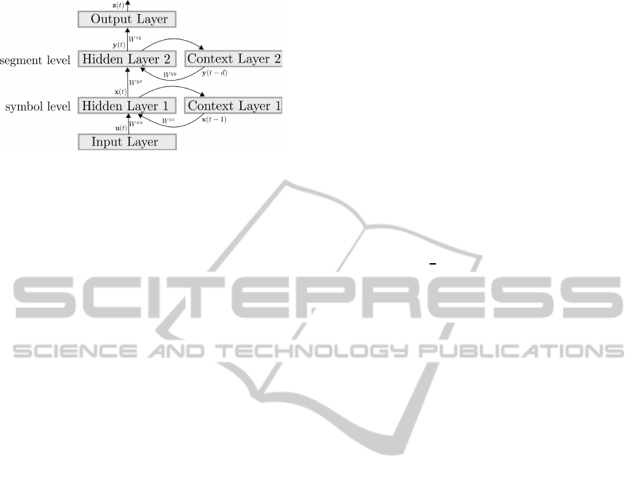
Figure 1: SMRNN topology.
2.1 Forward Processing in SMRNNs
We use the receiver-sender-notation to describe the
processing in the network. The upper index of the
weight matrices refer to the corresponding layer and
the lower index to the single units. For example, W
xu
ki
denotes the connection between the kth unit in hid-
den layer 1 (x) and the ith unit in the input layer (u)
(cf. Fig. 1). Moreover, f
net
is the transfer function of
the network and n
u
, n
x
, n
y
, n
z
are the number of units
in the input, hidden 1, hidden 2, and output layer.
The introduction of the parameter d on segment
level makes the main difference between a cascade
of SRNs and an SMRNN. It denotes the length of a
segment, which can be fixed or variable. The process-
ing of an input sequence starts with the initial symbol
level state x(0) and segment level state y(0). At the
beginning of a segment (segment head SH) x(t) is up-
dated with x(0) and input u(t). On other positions
x(t) is obtained from its previous state x(t − 1) and
input u(t). It is calculated by
x
k
(t) =
f
net
∑
n
x
j
W
xx
k j
x
j
(0) +
∑
n
u
i
W
xu
ki
u
i
(t)
, if SH
f
net
∑
n
x
j
W
xx
k j
x
j
(t − 1) +
∑
n
u
i
W
xu
ki
u
i
(t)
,
otherwise
(1)
where k = 1, . . . ,n
x
. The segment level state y(0)
is updated at the end of each segment (segment tail
ST) as
y
k
(t) =
f
net
∑
n
y
j
W
yy
kj
y
j
(t − 1) +
∑
n
x
i
W
yx
ki
x
i
(t)
,
if ST
y
k
(t − 1), otherwise
(2)
where k = 1,...,n
y
. The network output results in
forwarding the segment level state
z
k
(t) = f
net
n
y
∑
j
W
zy
kj
y
j
(t)
!
with k = 1,... ,n
z
.
(3)
While the symbol level is updated on a symbol by
symbol basis, the segment level changes only after d
symbols. At the end of the input sequence the seg-
ment level state is forwarded to the output layer to
generate the final output. The dynamics of an SM-
RNN processing a sequence is shown in Fig. 2.
2.2 Extension of BPTT for SMRNNs
In the following, we describe how to adapt online
BackpropagationThrough Time to SMRNNs. That is,
the error at the output at the end of a sequence is used
instantaneously for weight adaptation of the network.
Learning is based on minimizing the sum of squared
errors at the end of a sequence of N segments,
E(t) =
∑
n
z
k=1
1
2
(z
k
(t) − d
k
(t))
2
, if t = Nd
0, otherwise
(4)
where d
k
(t) is the desired output and z
k
(t) is the actual
output of the kth unit in the output layer.
The error is propagated back through the network
and also back through time to adapt the weights. Fur-
ther, it is not reasonable to keep the initial states
y(0) = f
net
(a
yy
(0)) and x(0) = f
net
(a
xx
(0)) fixed,
thus, the initial activations a
yy
(0) and a
xx
(0) are also
learned. Here, the upper index of the activations re-
fer to the corresponding layer and a lower index to
the single units. For example, a
yx
k
is the activation
at the kth unit in the hidden layer 2 that results from
connections from the hidden layer 1, which is simply
a
yx
k
(t) =
∑
n
x
i
W
yx
ki
x
i
(t).
The gradient of E(t) can be computed from the
injecting error
e
k
(t) = z
k
(t) − d
k
(t). (5)
Using the back propagation procedure we compute
the delta error. The δ
k
(t) is a short hand for ∂E(t)/∂a
k
representing the sensitivity of E(t) to small changes
of the kth unit activation. The deltas for the output
units δ
zy
, hidden layer 2 units δ
yy
, and hidden layer 1
units δ
yx
at the end of a sequence (t = Nd) are
δ
zy
k
(t) = f
′
net
(a
zy
k
(t))e
k
(t), (6)
δ
yy
k
(t) = f
′
net
(a
yy
k
(t))
n
z
∑
i=1
W
zy
ik
δ
zy
i
(t) (7)
δ
yx
k
(t) = f
′
net
(a
yx
k
(t))
n
z
∑
i=1
W
zy
ik
δ
zy
i
(t). (8)
At that point, we unroll the SMRNN on segment level
to propagate the error back in time. The state of the
hidden layer 2 changes only at the end of a segment
t = nd and n = 0,...,N − 1. Therefore, the delta error
for the hidden layer 2, and hidden layer 1 units results
IJCCI2012-InternationalJointConferenceonComputationalIntelligence
452
Figure 2: SMRNN dynamics for a sequence of three segments with fixed interval d. Processing on symbol level is described
by Eq. 1 and illustrated in the dashed squares. The segment level above, is processes as described by Eq. 2. Finally, Eq. 3
describes how the network output z is obtained for the sequence.
in
δ
yy
k
(nd) = f
′
net
(a
yy
k
(nd))
n
y
∑
i=1
W
yy
ik
δ
yy
i
((n+ 1)d), (9)
δ
yx
k
(nd) = f
′
net
(a
yx
k
(nd))
n
y
∑
i=1
W
yy
ik
δ
yy
i
((n+ 1)d). (10)
Once the computation was performed down to the be-
ginning of the sequence (t = 0), the gradient of the
weights and initial activation on segment level is com-
puted by
∆W
zy
ij
= δ
zy
i
(Nd)y
j
(Nd), (11)
∆W
yy
ij
=
N
∑
n=1
δ
yy
i
(nd)y
j
((n− 1)d), (12)
∆W
yx
ij
=
N
∑
n=2
δ
yx
i
(nd)x
j
((n− 1)d), (13)
∆a
yy
i
= δ
yy
i
(0). (14)
For the adaptation of the weights on symbol level we
apply the Backpropagation Through Time procedure
repetitively for every time step τ = 0,...,d for every
segment of the sequence. That is, for the end of a
segment (τ = d)
δ
xx
k
(d) = f
′
net
(a
xx
k
(d))
n
y
∑
i=1
W
yx
ik
δ
yx
i
(d), (15)
δ
xu
k
(d) = f
′
net
(a
xu
k
(d))
n
y
∑
i=1
W
yx
ik
δ
yx
i
(d), (16)
and for τ < d we get
δ
xx
k
(τ) = f
′
net
(a
xx
k
(τ))
n
x
∑
i=1
W
xx
ik
δ
xx
i
(τ+ 1), (17)
δ
xu
k
(τ) = f
′
net
(a
xu
k
(τ))
n
x
∑
i=1
W
xx
ik
δ
xx
i
(τ+ 1). (18)
When the computation was performed to the begin-
ning of a segment (τ = 0), the gradient of the weights
and initial activation on symbol level is computed by
∆W
xx
ij
=
d
∑
τ=1
δ
xx
i
(τ)x
j
(τ− 1), (19)
∆W
xu
ij
=
d
∑
τ=2
δ
xu
i
(τ)u
j
(τ− 1), (20)
∆a
xx
i
= δ
xx
i
(0). (21)
Note that the sums in Eq. 13 and 20 start at n = 2
and τ = 2, respectively. This is due to the fact, that at
time t = 0 the hidden layer 2 has no input from hidden
layer 1 and further, hidden layer 1 has no input from
the input layer (cf. Fig. 2).
The computed gradients can be used right away to
change the networks weights and initial activations to
˜
W
ij
= W
ij
− α∆W
ij
+ η∆
′
W
ij
(22)
with a learning rate α and the momentum term η. The
value ∆
′
W
ij
represents the change of W
ij
in the previ-
ous iteration. Figure 3 illustrates the error flow in the
SMRNN for one sequence of length Nd.
2.3 Information Latching Problem
Typically dynamic systems change the output on cur-
rent or immediate past inputs. Nevertheless, it is of-
ten desired that even inputs that occurred much ear-
lier affect the system’s output. The information latch-
ing problem was designed to test a system’s ability
to model dependencies of the output on earlier inputs
(Bengio et al., 1994). In this context, “information
latching” refers to the storage of information in the
internal states of the system over some period of time.
The task is to distinguish two classes of sequences
where the classC of the sequence i
1
,i
2
,...,i
T
depends
on the first L items
C(i
1
,i
2
,. .., i
T
) = C(i
1
,i
2
,. .., i
L
) ∈ {0,1} with L < T
(23)
For our experiments the class-defining start of a
sequence had a fixed length of L = 50. To test the
ExtensionofBackpropagationthroughTimeforSegmented-memoryRecurrentNeuralNetworks
453
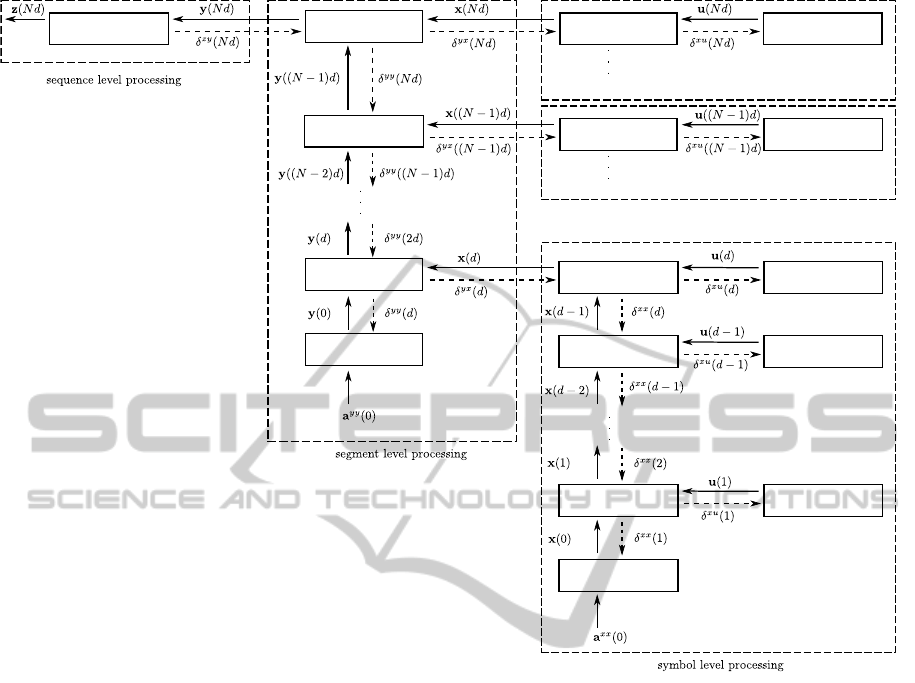
Figure 3: Errorflow of the eBPTT algorithm in an SMRNN for a sequence of length Nd. The solid arrows indicate the
development of the states of the layers in the network. The dashed arrows show the propagation of the error back through the
network and back through time.
networks ability to store the initial inputs over an arbi-
trary period of time, we gradually increased the length
of the sequence T. The sequences were generated
from an alphabet of 26 letters (a-z), such that the num-
ber of input neurons was 26 (1-of-N coding). A se-
quence was considered to be class C = 1 if the items
i
1
,i
2
,...,i
L
match a predefined string s
1
,s
2
,...,s
L
,
otherwise it was class C = 0. All items i of a sequence
that were not predefined were chosen randomly from
the alphabet.
For each sequence length T we created two sets
of sequences for training and testing. With increasing
length of the sequences T the set of training and test
samples was enlarged to ensure generalisation.
3 RESULTS
For every sequence length T we trained 100 networks
with eRTRL (Chen and Chaudhari, 2009) and eBPTT,
respectively. This was done to determine the algo-
rithms’ ability to learn the task in general. In every
epoch the sequences of the training set were shown in
a random order.
The networks’ configuration and the size of the
training/test sets are adopted from (Chen and Chaud-
hari, 2009) where SMRNNs and SRNs are compared
on the information latching problem. Accordingly,
the SMRNNs are comprised of n
u
= 26 input units,
n
x
= n
y
= 10 units in the hidden layers, and one out-
put unit (n
z
= 1). Further, the length of a segment
was set to d = 15 and the sigmoidal transfer function
f
net
(x) = 1/(1 + exp(−x)) was used for the hidden
and output units. The input units simply forwarded
the input data which were ∈ {−1, 1}. Initial weights
were set to uniformly distributed random values in the
range of (−1,1).
Learning rate and momentum for each algo-
rithm were chosen after testing 100 networks on
all combinations α ∈ {0.1,0.2, . . .,0.9} and η ∈
{0.1, 0.2,...,0.9} on the shortest sequence T = 60.
IJCCI2012-InternationalJointConferenceonComputationalIntelligence
454

The combinations that yielded the highest mean ac-
curacy on the test set were chosen for the experiment,
that is α = 0.1, η = 0.4 for eRTRL and α = 0.6,
η = 0.5 for eBPTT.
Training was stopped when the mean squared er-
ror of an epoch fell below 0.01 and thus, the net-
work was considered to have successfully learned the
task. For other cases training was cancelledafter 1000
epochs. Table 1 shows the results for eRTRL and
eBPTT for sequences of length T from 60 to 130.
The column for the number of successfully trained
networks (#suc) in Tab. 1 clearly shows a decrease
for eBPTT with the length of the sequences T. On
the other hand, nearly all networks were trained suc-
cessfully with eRTRL. Therefore, we can state that
eRTRL is generally able to cope better with longer
ranges of output dependencies than eBPTT.
The pure mean number of epochs (#eps) that were
needed for training is somewhat misleading. Over the
whole experiment eBPTT needs an average of 243.3
epochs for successful training while eRTRL needs
only 67.1 epochs. It is important to note that this does
not indicate that eRTRL training takes less time than
eBPTT. The high computational complexity of Real-
Time Recurrent Learning (O (n
4
)), and therefore also
of eRTRL, results in a much longer computation time
for a single epoch compared to eBPTT. This becomes
more and more evident with increasing network size.
Figure 4 shows the time that is needed to train an SM-
RNN for 100 epochs (T = 60, set size 50) depending
on the number of neurons in the hidden layers
1
. For
a considerable big network with n
x
= n
y
= 100 the
training took about 3 minutes with eBPTT and 21.65
hours with eRTRL.
0 200 400 600 800 1000
0
5
10
15
20
22
number of neurons in hidden layers n
x
= n
y
time for training in hours
eBPTT
eRTRL
Figure 4: Computation time for training depending on the
number of neurons in the hidden layers of the network.
Training lasted 100 epochs of 50 sequences of length T =
60.
1
Both algorithms were implemented in Matlab. Training
was done on a AMD Opteron 8222 (3GHz), 8GB RAM,
CentOS, Matlab R2011b (7.13.0.564) 64-bit.
The third column in Tab. 1 shows the performance
of successfully trained networks on the test set (Acc.).
For eBPTT we could observe higher accuracies than
for eRTRL. It is also reflected by the overall accuracy
of 96.8% for eBPTT compared to 89.2% for eRTRL.
This implies, that successful learning with eBPTT
guaranteed better generalisation.
4 DISCUSSION
Even though eRTRL was generally better able to cope
with the latching of information over longer periods
of time, the networks that finally learned the task with
eBPTT showed higher accuracies on the test set.
Altogether, the question which learning algorithm
to use for a specific task strongly depends on the char-
acter of the problem at hand. For small networks, as
used for the experiment in Tab. 1, the choice depends
on the timespan that has to be bridged. If we expect
the output to be dependent on inputs that are com-
paratively shortly ago (T = 60,.. . , 100) eBPTT pro-
vides the better choice. There is a high chance for a
successful training of the network with a good gen-
eralisation. When the outputs depend on inputs that
appeared long ago (T > 130), the eRTRL algorithm
provides the better solution. It guarantees a success-
ful network training where eBPTT could hardly train
the network.
In real world problems, as speech recognition,
handwriting recognition or protein secondary struc-
ture prediction the data to be classified has not such
a compact representation as the strings in the infor-
mation latching task. To be able to learn from such
data the network size, that is, number of processing
units, has to be increased. As shown in Fig. 4, eRTRL
becomes simply impractical for large networks (train-
ing time: 3 minutes with eBPTT in contrast to 21.65
hours with eRTRL / n
x
= n
y
= 100). In these cases,
eBPTT becomes the only viable choice of a training
algorithm.
In future, the combination of both learning algo-
rithms might be a possibility to overcome the draw-
backs of both methods. It could reduce the compu-
tational complexity of eRTRL and increase eBPTT’s
ability to learn long-term dependencies.
ACKNOWLEDGEMENTS
The authors acknowledge the support provided by
the Transregional Collaborative Research Centre
SFB/TRR 62 “Companion-Technology for Cognitive
ExtensionofBackpropagationthroughTimeforSegmented-memoryRecurrentNeuralNetworks
455

Table 1: Information latching problem with increasing sequence length T and fixed predefined string (L = 50). The size of
sets for training/testing was increased too. 100 SMRNNs with parameters n
x
= n
y
= 10, d = 15 were trained on each sequence
length. The number of networks that learned the task (#suc of 100) and the mean value of number of epochs (#eps) is shown
together with the mean accuracy (Acc.) of successful networks on the test set and its standard deviation (Std. Dev.).
T set size
eBPTT eRTRL
#suc #eps Acc. Std. Dev. #suc #eps Acc. Std. Dev.
60 50 79 230.6 0.978 0.025 100 44.3 0.978 0.025
70 80 58 285.7 0.951 0.047 100 63.9 0.861 0.052
80 100
61 215.2 0.974 0.024 100 66.2 0.862 0.088
90 150 48 240.4 0.951 0.123 100 52.4 0.940 0.044
100 150
43 241.4 0.968 0.018 100 82.1 0.778 0.065
110 300 36 250.0 0.977 0.049 100 69.6 0.868 0.052
120 400
17 305.4 0.967 0.050 100 56.7 0.950 0.040
130 500 14 177.6 0.978 0.017 96 101.4 0.896 0.078
mean 243.3 0.968 0.044 67.1 0.892 0.056
Technical Systems” funded by the German Research
Foundation (DFG).
REFERENCES
Bengio, Y., Simard, P., and Frasconi, P. (1994). Learn-
ing long-term dependencies with gradient descent is
difficult. IEEE Transactions on Neural Networks,
5(2):157–166.
Chen, J. and Chaudhari, N. S. (2009). Segmented-memory
recurrent neural networks. IEEE Transactions Neural
Networks, 20(8):1267–1280.
Elman, J. L. (1990). Finding structure in time. Cognitive
Science, 14(2):179–211.
Gl¨uge, S., B¨ock, R., and Wendemuth, A. (2011).
Segmented-memory recurrent neural networks ver-
sus hidden markov models in emotion recognition
from speech. In International Conference on Neural
Computation Theory and Applications (NCTA 2011),
pages 308–315, Paris.
Werbos, P. (1990). Backpropagation through time: what
it does and how to do it. Proceedings of the IEEE,
78(10):1550 –1560.
Williams, R. J. and Zipser, D. (1989). A learning algo-
rithm for continually running fully recurrent neural
networks. Neural Computation, 1(2):270–280.
Williams, R. J. and Zipser, D. (1995). Gradient-based
learning algorithms for recurrent networks and their
computational complexity, pages 433–486. L. Erl-
baum Associates Inc., Hillsdale, NJ, USA.
IJCCI2012-InternationalJointConferenceonComputationalIntelligence
456
