
The Difficulty of Path Traversal in Information Networks
Frank W. Takes and Walter A. Kosters
Leiden Institute of Advanced Computer Science (LIACS), Leiden University
P.O. Box 9512, 2300 RA Leiden, The Netherlands
Keywords:
Information Networks, Path Traversal, Wikipedia.
Abstract:
This paper introduces a set of classification techniques for determining the difficulty — for a human — of
path traversal in an information network. In order to ensure the generalizability of our approach, we do not
use ontologies or concepts of expected semantic relatedness, but rather focus on local and global structural
graph properties and measures to determine the difficulty of finding a certain path. Using a large corpus of over
two million traversed paths on Wikipedia, we demonstrate how our techniques are able to accurately assess
the human difficulty of finding a path between two articles within an information network.
1 INTRODUCTION
Searching and navigating through structured informa-
tion such as Wikipedia, a social network or the web,
has become an aspect of people’s daily lives. In this
paper we will analyze the way in which humans tra-
verse structured data in search of a specific piece of
information. The motivation for this work comes
from the fact that understanding the difficulty of path
traversal may lead to a better understanding of human
search behavior in general (Hsieh-Yee, 2001), possi-
bly improving the strategy of intelligent search algo-
rithms. Understanding the aspects which complicate
path traversal may also help to improve the structure
of the linked data itself (Bizer et al., 2009).
Although search engines can often help to find
the content within a structured dataset that the user
is looking for, sometimes search engine performance
does not exactly meet the user’s needs (Teevan et al.,
2004), for example because the required page is lo-
cated within the so-called “Deep Web” (He et al.,
2007). In such cases, the user will have to reach the
correct article by traversing hyperlinks and forming a
path towards the correct piece of information. We will
study this type of path traversal by analyzing over two
million paths traversed by (human) users of the well-
known online encyclopedia Wikipedia. The path data
was gathered from The Wiki Game, an online game
in which the user is assigned the task of connecting
two given random articles on Wikipedia by follow-
ing the clickable links within the Wikipedia articles.
In turns out that humans, especially after some prac-
tice, are often able to complete this task in less than
10 clicks. This is actually a quite remarkable accom-
plishment, because even though a standard backtrack-
ing algorithm is certainly able to match or even beat
humans in terms of path length, a human instead does
not use millions of backtracking steps, but rather re-
lies on background knowledge in terms of expected
semantic relatedness (Kentsch et al., 2011). However,
incorporating such extensive knowledge into an algo-
rithm for classifying path difficulty, for example via
ontologies, may in large networks such as Wikipedia
be too complex.
Instead, we will propose a range of local and
global structural network properties and measures as
indicators for the difficulty of connecting two articles.
An advantage of considering structural features is that
they capture the direct relationship between the con-
cepts within the network, independent of which ex-
act information network is studied, ensuring the gen-
eralizability of the approach. Also, structural prop-
erties are relatively easy to compute, and do not re-
quire prior knowledgeabout the dataset. Furthermore,
while both the content as well as the linking structure
of Wikipedia are subject to change, the classifiers that
we propose will only be affected by the second type
of change.
The rest of this paper is organized as follows.
First, Section 2 describes some concepts, our datasets,
and defines our main problem statement. Related
work is discussed in Section 3. We analyze and com-
pare the techniques for assessing the difficulty of path
traversal, at a local as well as on a global scale, in
Section 4 and 5, respectively. Section 6 concludes.
138
W. Takes F. and A. Kosters W..
The Difficulty of Path Traversal in Information Networks.
DOI: 10.5220/0004104201380144
In Proceedings of the International Conference on Knowledge Discovery and Information Retrieval (KDIR-2012), pages 138-144
ISBN: 978-989-8565-29-7
Copyright
c
2012 SCITEPRESS (Science and Technology Publications, Lda.)

2 PRELIMINARIES
In this section we first discuss various concepts and
definitions, after which we describe our two main
datasets. Next we formulate our problem statement
and verification approach.
2.1 Concepts & Definitions
Our structured data will be represented by a directed
graph G(V, E) with n = |V| nodes and m = |E| links.
When we talk about a path between two nodes u,v ∈
V, we mean a sequence consisting of at least two
nodes, starting at u and ending at v, where there is a
link from each node to the next node in the sequence.
A shortest path between two nodes u,v ∈ V is a path
of length ℓ ≥ 1 between u and v for which there is no
other path from u to v of length smaller than ℓ. The
length of such a shortest path, or in short the distance,
is denoted by d(u,v). If there is no (shortest) path,
then d(u,v) = ∞, and of course there can be multiple
(shortest) paths connecting two nodes. Because our
graph is directed, it can happen that d(u,v) 6= d(v, u).
We define the indegree indeg(v) of a node v ∈ V as the
number of links pointing to node v, and similarly, the
outdegree outdeg(v) as the number of links pointing
from node v to some other node.
2.2 Wikipedia
Wikipedia (
http://www.wikipedia.org
) accord-
ing to its own definition, “is a free, web-based, collab-
orative, multilingual encyclopedia project with over
3.9 million articles in English alone”. Considering
solely the content of the articles and the links it con-
tains, Wikipedia can be seen as a large directed graph,
where each node represents an article, and each di-
rected link a hyperlink within the source article point-
ing to the target article. In this study we will use
the August 2011 English dataset of Wikipedia from
DBpedia (Auer et al., 2007), from which we only
consider the so-called “pagelinks” to other Wikipedia
articles, so we exclude links to external websites or
other special pages. After some pruning and clean-
ing, the Wikipedia graph has statistics as presented in
Table 1.
We note that the edge-to-node ratio, diameter, the
effective diameter (the 90-th percentile of the cumula-
tive distribution of shortest path lengths), the average
node-to-node distance (sampled over 10,000 node
pairs) and the size of the largest (weakly) connected
component (WCC) are consistent with that of other
small world networks (Watts and Strogatz, 1998). We
also confirmed the power-law node degree distribu-
Table 1: Wikipedia dataset.
Articles (n) 3,464,902
Directed links (m) 82,019,786
Largest WCC 99.9%
Average indegree 26
Average outdegree 22
Average distance (d) 4.81
Effective diameter 7
Diameter 11
tion for our Wikipedia dataset.
2.3 The Wiki Game
The Wiki Game (
http://thewikigame.com
) is an
online game in which, starting from a certain source
article, the main objective is to reach the goal arti-
cle by repeatedly clicking links on the current arti-
cle’s page. We will focus on the “speed-race”-games,
in which the task is to connect two given random
Wikipedia articles in as few steps as possible, as
quickly as possible, with a time limit of 120 seconds.
As an example of a path traversal task, consider the
path from the Wikipedia article on MP3 to the article
on Northern Ireland. An actual (computed) shortest
path of length 3 runs subsequently via the articles on
the United States and Ice Hockey (see Figure 1). Hu-
man users attempting to find a path tend to know that
Northern Ireland is somewhere in Europe, so from the
article on MP3 they first find their way to an article
related to Europe, for example via the page on the In-
ternet which is a direct link from the article on MP3.
Next, they will for example navigate to the article on
the United Kingdom, from where they find the article
on Northern Ireland. Some users take another detour
on the way, for example via the pages Republic of Ire-
land and Ireland (island).
Our dataset T consists of 407,268 games (or
tasks) and a total of 2,278,986 user-generated paths.
A task is essentially a (start, goal)-pair inbetween
which a path has to be formed. For each of these
tasks we have a list of paths generated by the (fully
anonymized) users, of which little less than one third
(28.0%) was successful. The data was filtered to ex-
clude non-serious attempts (more than 40 clicks per
task, or no clicks at all).
Figure 2 further clarifies the distribution of short-
est and user-generated path lengths. We note that even
though shortest paths of length greater than 6 exist
within Wikipedia, none of these tasks were included
in our database of attempted tasks. Most tasks have
a shortest path length somewhere between 2 and 4
(red line, ▽). Figure 2 shows how the distribution
of the successful user-generated paths (blue line, ♦)
has a fat tail and follows the same distribution as that
TheDifficultyofPathTraversalinInformationNetworks
139
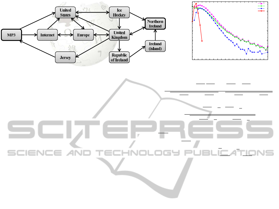
Figure 1: Sample of a fictive Wikipedia graph.
1e-06
1e-05
0.0001
0.001
0.01
0.1
1
2 4 6 8 10 12 14 16 18 20 22 24 26 28 30 32 34 36 38 40
relative frequency
path length
all user-generated paths
failed user-generated paths
succesful user-generated paths
shortest path length over all tasks
Figure 2: Path lengths (relative frequency).
of the shortest paths, but with an average path length
that is roughly 2 times larger than the shortest path
length (between 5 and 7). The distribution of the path
length over all user-generated paths (purple line, ) is
clearly dominated by the failed paths (green line, ×)
and follows a fat-tailed power law, indicating that
people frequently “fail” early in the process.
2.4 Problem Definition
Our main goal is to assess the difficulty of finding a
path between two nodes in a directed graph:
Problem 1. Given a directed graph G(V,E) and
nodes u,v ∈ V, can we assign a function value
f(u,v) ∈ [0;1] indicating the difficulty of finding a
path from u to v?
In this paper we will consider various approaches
(or difficulty classifiers) of assigning such a function
value. We evaluate the quality of an approach based
on a comparison with the results obtained by the users
on tasks from The Wiki Game.
For each of the user-generated paths of a certain
task t ∈ T we know whether or not the path was suc-
cessfully formed, allowing us to define the average
percentage of success g(t) ∈ [0;1] for task t, which
will serve as a ground truth for assessing the quality
of our classifiers.
A classifier f can assign a function value f(t) to
all tasks t ∈ T, which allows us to create a partition
{T
1
,T
2
,... ,T
q
} of the set of tasks T. The partitioning
is done in such a way that the tasks in each T
i
have
the same function value (range), so that the (average)
function value of the tasks in T
i
is always greater than
the average function value of tasks in T
i−1
, and where
every T
i
is maximal in size. The partitions can be used
to define q difficulty levels for The Wiki Game.
The overall quality of a classification measure will
be determined by computing both the Pearson corre-
lation coefficient c( f,g) as well as the Spearman rank
correlation coefficient rc( f,g) of f and g, defined as:
c( f, g) =
q
∑
i
f(i) g(i) −
∑
i
f(i)
∑
i
g(i)
q
q
∑
i
f(i)
2
− (
∑
i
f(i))
2
q
q
∑
i
g(i)
2
− (
∑
i
g(i))
2
rc( f, g) =
∑
i
( f(i) − f)(g(i) − g)
r
∑
i
f(i) − f
2
∑
i
g(i) − g
2
Here, f(i) is equal to the average function value f(t)
of paths t ∈ T
i
, g(i) is the average percentage of suc-
cess of the paths in T
i
, and f and g are equal to
the average value over all i of f (i) and g(i), respec-
tively. The correlation coefficient measures the extent
to which the two attributes f and g are correlated. If
we want a task at a certain difficulty level to always be
harder than a task at the previous level, then we pri-
marily aim for a high rank correlation coefficient, as it
describes the extent to which the relation between the
classifier output and path difficulty can be described
using a monotonic function.
We call a measure correlated with path difficulty
if it has a correlation larger than 0.8 or smaller than
−0.8. For simplicity, we denote the correlation and
rank correlation coefficient by c and rc, respectively.
3 RELATED WORK
The structure behind Wikipedia has been analyzed in
great detail, addressing tasks such as improving the
linking structure (Milne and Witten, 2008) and au-
tomatic disambiguation of articles (Hu et al., 2009).
Patterns within clickpaths have also been analyzed
extensively, and have proven useful for tasks such as
page prediction (Agarwal et al., 2010). These patterns
are often found within clickstreams from the web,
where there is a great deal of “noise”, by which we
refer to duplicate, false or untrusted information. An
advantage of studying paths on Wikipedia is that due
to the active user base, there is much less noise. Using
a dataset similar to ours, a comparison between auto-
matic and human navigation in Wikipedia was made
in (West and Leskovec, 2012a). An extensive analysis
KDIR2012-InternationalConferenceonKnowledgeDiscoveryandInformationRetrieval
140
of the path data was done and methods for predicting
the target page were introduced (West and Leskovec,
2012b). To the best of our knowledge, the isssue of
path difficulty has so far been unaddressed.
4 LOCAL DIFFICULTY
MEASURES
In this section we consider local difficulty measures
that depend solely on a node and its neighborhood, in
our case the Wikipedia article and its linked or linking
articles.
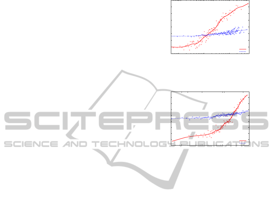
4.1 Degree Measures
Having a large number of outgoing links for a cer-
tain node is likely to make it easier to directly reach
a larger part of the graph from that particular node.
Similarly, we expect that the number of incoming
links of a node will probably make it relatively more
easy to reach that node from any other node. We will
verify the actual influence of these two measures by
analyzing q = 100 ranges of goal article’s indegrees
and start article’s outdegrees. The results are depicted
in Figure 3, and a Bezier curve is drawn to get a bet-
ter idea of the overall correlation. We observe no real
significant correlation with the starting article’s out-
degree (c = 0.637 and rc = 0.789). However, a strong
correlation (c = 0.850 and rc = 0.960) is noticeable
with respect to the indegree of the goal article and
the actual percentage of success. Apparently, the in-
degree of the goal article is of great influence to the
difficulty of finding a certain path, whereas the out-
degree of the starting node does not appear to play a
very significant role. Because the graph is stored as
an adjacency list, degree measures can be computed
in O(1).
4.2 Neighborhood Measures
Extending the degree measure, we define the ℓ-
neighborhood N
ℓ
(v) of a node v ∈ V as the set of
nodes with distance at most ℓ from v, more specifi-
cally: N
ℓ
(v) = {w ∈ V | d(v,w) ≤ ℓ}. Similarly, we
can define N
′
ℓ
(v) = {u ∈ V | d(u,v) ≤ ℓ}, the reverse
neighborhood, which is the set of all articles u with
distance at most ℓ to v. The ℓ-neighborhoodsize is the
number of nodes in the neighborhood of v, denoted
by |N
ℓ
(v)|, and similarly we can define the reversed
ℓ-neighborhood size |N
′
ℓ
(v)|. The functionality of this
measure can be explained by looking at the example
graph in Figure 1. There, the article on Ice Hockey
0.3
0.35
0.4
0.45
0.5
0.55
0.6
0.65
0.7
100 1000 10000
10 100 1000
percentage successful
goal indegree
start outdegree
goal indegree
start outdegree
Figure 3: Start outdegree and goal indegree (horizontal
axes, logarithmic) vs. percentage successful (vertical axis).
0.25
0.3
0.35
0.4
0.45
0.5
0.55
0.6
0.65
0.7
1000 10000 100000 1e+06
1000 10000
percentage successful
goal reversed 2-neighborhood size
start 2-neighborhood size
goal reversed 2-neighborhood size
start 2-neighborhood size
Figure 4: Start & goal 2-neighborhood measures (horizontal
axes, logarithmic) vs. percentage successful (vertical axis).
and the article on Ireland (island) both have an inde-
gree of 1, while intuitively, but also based on the de-
gree of the neighbors, Ice Hockey seems much easier
to reach than Ireland (island), which is nicely reflected
by the reversed 2-neighborhood size, as |N
′
2
(Ireland
(island))| = 3 and |N
′
2
(Ice Hockey)| = 6.
Figure 4 shows q = 100 intervals of the goal ar-
ticle’s reversed 2-neighborhood, again compared to
the success percentage, and strong correlation coef-
ficients (c = 0.915 and rc = 0.978) can be observed.
We notice how for the hardest (g(t) < 0.35) tasks in
the database, looking beyond the indegree apparently
helps to increase the amount of monotonicity. Again,
the starting node’s 2-neighborhood did not appear to
be relevant (c = 0.397 and rc = 0.492).
Even though in some graphs it makes sense to look
at (reverse) neighborhoods larger than ℓ = 2, in our
dense Wikipedia graph, considering more than the 2-
neighborhood will quickly yield the entire graph, and
indeed, correlation coefficients lower than 0.5 are ob-
served when considering larger neighborhoods. We
note that the neighborhood measures discussed here
can be computed in O((m/n)
ℓ−1
) time per task. The
average node indegree (or outdegree), (m/n), is be-
tween 20 and 30, still allowing for quick computation
of this local measure, especially for ℓ = 2.
Concluding this section on local measures, we can
say that the reversed 2-neighborhood size is the best
TheDifficultyofPathTraversalinInformationNetworks
141

indicator for path difficulty, whereas measures related
to the starting article do not appear to be effective.
This can be explained by considering the small-world
property of the Wikipedia: with relatively few steps
it is possible to reach a large portion of the graph via
so-called hubs. The user will often find his way to a
hub node very quickly, from where the actual search
for the goal node starts, making the first part of the
search of little influence in general.
5 GLOBAL DIFFICULTY
MEASURES
In contrast with the previous section, we will now
look at global properties of the nodes, meaning
that we look at actual paths and global central-
ity measures, using knowledge about the entire
graph. Though possibly better in terms of prediction
strength, the computation time of global measures is
longer, typically O(m) per task.
5.1 Path Length
As mentioned in Section 2 and shown in Figure 2, the
distribution of user-generated path lengths follows the
same type of distribution as that of the actual short-
est paths, suggesting a correlation between the two.
Whereas we were able to aggregate our local mea-
sures from the previous section into q = 100 inter-
vals, in case of shortest path length we only have 6
different values. In Figure 6, the solid line shows for
each actual distance the percentage of successful hu-
man paths. This shows a strong correlation coeffi-
cient of c = −0.957 between the computed shortest
path length and the percentage of successful paths,
and an obvious rank correlation of rc = −1.000. A
clear downside of this measure is the fact that we can
only define q = 6 different difficulty levels.
5.2 Number of Shortest Paths
We may also choose to look at the number of short-
est paths σ(u,v) between the start and goal article u
and v. Intuitively, if there is only one shortest path
from the start node to the end node, the task will
be much harder compared to when there would have
been thousands of shortest paths. Luckily, comput-
ing actual shortest path lengths is easy, as σ(u,u) = 1
and σ(u, v) =
∑
w∈B(u,v)
σ(u,w) with B(u,v) = {w ∈
N
′
1
(v) : d(u,v) = d(u,w) + 1} (Brandes, 2001). The
number of shortest paths showed no significant corre-
lation with path difficulty, which is understandable: a
path of length 2 with 20 possible shortest paths is ex-
pected to be much easier to find than a path of length
4 with 20 shortest paths. So we propose to combine
the distance with the number of shortest paths:
dsp(u,v) = d(u,v) + α
1−
logσ(u, v)
max
w,z∈V
(logσ(w,z))
The reason why we take the log of σ(u,v) is motivated
by Figure 5, where the thick lines indicate how the
distribution of the number of shortest paths for each
shortest path length decreases logarithmically. The
parameter α ≥ 0 essentially defines the amount of fo-
cus on the number of shortest paths. If this parameter
is set to 1, then a path of length 4 with only 1 possi-
ble shortest path is assumed to be easier to find than
a path of length 5 with 2000 different shortest paths.
After some parameter tuning we obtained the best re-
sults for α = 1.5, where we observe again a strong
correlation of c = −0.895 and rc = −0.876 with path
difficulty. The results are depicted in Figure 6.
5.3 Shortest Paths Uniqueness
To further refine the measure from the previous sec-
tion, we propose to look at the number of distinct
nodes that occur within these shortest paths. This
measure is based on the intuition that shortest paths
quickly overlap, and that the extent to which paths
overlap may influence the difficulty of a path finding
10
100
1000
10000
100000
200 400 600 800 1000 1200 1400
frequency
number of shortest paths / unique nodes on shortest paths
distance 2 - shortest paths
distance 3 - shortest paths
distance 4 - shortest paths
distance 5 - shortest paths
distance 6 - shortest paths
distance 2 - unique nodes
distance 3 - unique nodes
distance 4 - unique nodes
distance 5 - unique nodes
distance 6 - unique nodes
Figure 5: Distribution of number of shortest paths and num-
ber of unique nodes on these paths for each distance.
0
0.1
0.2
0.3
0.4
0.5
0.6
0.7
1 2 3 4 5 6 7
percentage successful
distance / distance + number of shortest paths
distance
distance + number of shortest paths
distance + shortest paths uniqueness
Figure 6: Various global measures (horizontal axis) vs. per-
centage successful (vertical axis).
KDIR2012-InternationalConferenceonKnowledgeDiscoveryandInformationRetrieval
142

task. For example, in Figure 1, the 3 shortest paths of
length 3 from MP3 to United Kingdom run through a
total of 4 different nodes: United States, Internet, Eu-
rope and Ice Hockey.The maximum number of unique
nodes on 3 shortest paths of length 3 is 6 (3 times 2
unique intermediary nodes). Somewhat inspired by
betweenness centrality, we propose to divide the num-
ber of nodes on the actual shortest paths by the maxi-
mum possible number of intermediary nodes, a mea-
sure which we will call shortest paths uniqueness. In
our example this results in a score of
4
6
≈ 0.67. We
will incorporate this measure along with the distance
in the difficulty classifier defined as:
dusp(u,v) = d(u,v)+β
1−
log(ψ(u,v))
log(d(u,v) × σ(u, v))
Here, ψ(u,v) is a function that returns the number of
distinct nodes on the shortest paths between u and v.
The used values are again logarithmic as a result of
the distribution of the number of unique nodes on the
shortest paths, depicted by the various thin lines in
Figure 5. The parameter β ≥ 0 indicates the amount of
focus on the number of distinct nodes over all shortest
paths, and best results were obtained for β = 1.75.
The performance of the measure is displayed by
the dotted line in Figure 6, showing a correlation of
c = −0.924 and rc = −0.925, demonstrating how
shortest paths uniqueness is a good refinement of the
global difficulty indicator based solely on distance.
6 CONCLUSIONS
Throughout this paper we have proposed and ana-
lyzed a range of techniquesfor classifying path traver-
sal difficulty in information networks. The results
are summarized in Table 2. Local measures related
to the goal article, such as the reversed neighborhood
size, appear to be most effective, whereas local prop-
erties of the source article appear to be of little in-
fluence to path difficulty. Apparently, a user tends to
quickly find his way to a hub node, from where the ac-
tual search process starts. As for the global measures
considered in this work, the distance between two
articles, though limited in range, is a good measure
of difficulty. Incorporating the percentage of unique
nodes over all shortest paths results in a global clas-
sifier with slightly better performance, but due to the
higher complexity of global measures, one may favor
the local classifiers in a practical application such as
The Wiki Game, where the difficulty classifiers could
be used to allow users to select a difficulty level.
In future work we would like to include more
article-specific information, such as the article’s link
Table 2: Summary of correlation coefficients (c), rank cor-
relation coefficients (rc) and complexity per task t = (u, v)
of the proposed difficulty classifiers for q difficulty classes.
Classifier Complexity q c rc
indeg(v) O(1) 100 0.850 0.960
outdeg(u) O(1) 100 0.637 0.789
|N
′
2
(v)| O(m/n) 100 0.915 0.978
|N
2
(u)| O(m/n) 100 0.397 0.492
d(u, v) O(m) 6 −0.957 −1.000
dsp(u,v) O(m) 100 −0.895 −0.876
dusp(u,v) O(m) 100 −0.924 −0.925
density, which loosely represents the branching fac-
tor. We also want to analyze a user’s frequent sub-
paths, which may help us to obtain a better under-
standing of the search process of a certain user or
group of similar users, possibly allowing us to per-
sonalize the difficulty indicators.
ACKNOWLEDGEMENTS
This research is part of the NWO COMPASS project
(#612.065.926). We thank A. Clemesha for the data.
REFERENCES
Agarwal, R., Veer Arya, K., and Shekhar, S. (2010). An
architectural framework for web information retrieval
based on user’s navigational pattern. In Proceedings
of the 5th International Conference on Industrial and
Information Systems, pages 195–200.
Auer, S., Bizer, C., Kobilarov, G., Lehmann, J., Cyganiak,
R., and Ives, Z. (2007). DBpedia: A nucleus for a
web of open data. In Proceedings of 6th International
Semantic Web Conference, pages 722–735.
Bizer, C., Heath, T., and Berners-Lee, T. (2009). Linked
data-the story so far. International Journal on Seman-
tic Web and Information Systems, 5(3):1–22.
Brandes, U. (2001). A faster algorithm for between-
ness centrality. Journal of Mathematical Sociology,
25(2):163–177.
He, B., Patel, M., Zhang, Z., and Chang, K. (2007). Ac-
cessing the deep web. Communications of the ACM,
50(5):94–101.
Hsieh-Yee, I. (2001). Research on web search behavior.
Library & Information Science, 23(2):167–185.
Hu, J., Wang, G., Lochovsky, F., Sun, J., and Chen,
Z. (2009). Understanding user’s query intent with
Wikipedia. In Proceedings of the 18th International
World Wide Web Conference, pages 471–480.
Kentsch, A. M., Kosters, W., van der Putten, P., and
Takes, F. (2011). Exploratory recommendations us-
ing Wikipedia’s linking structure. In Proceedings of
the 20th Belgian Netherlands Conference on Machine
Learning, pages 61–68.
TheDifficultyofPathTraversalinInformationNetworks
143

Milne, D. and Witten, I. (2008). Learning to link with
Wikipedia. In Proceedings of the 17th Conference on
Information and Knowledge Management, pages 509–
518.
Teevan, J., Alvarado, C., Ackerman, M., and Karger, D.
(2004). The perfect search engine is not enough: A
study of orienteering behavior in directed search. In
Proceedings of the SIGCHI Conference on Human
Factors in Computing Systems, pages 415–422.
Watts, D. and Strogatz, S. (1998). Collective dynamics of
small-world-networks. Nature, 393(6684):440–442.
West, R. and Leskovec, J. (2012a). Automatic versus human
navigation in information networks. In Proceedings of
the International Conference on Weblogs and Social
Media. To appear.
West, R. and Leskovec, J. (2012b). Human wayfinding
in information networks. In Proceedings of the 21st
World Wide Web Conference, pages 619–628.
KDIR2012-InternationalConferenceonKnowledgeDiscoveryandInformationRetrieval
144
