
Categorization of Very Short Documents
Mika Timonen
VTT Technical Research Centre of Finland, PO Box 1000, 02044 Espoo, Finland
Department of Computer Science, University of Helsinki, Helsinki, Finland
Keywords:
Category Distribution, Feature Weighting, Short Document Categorization, SVM, Text Categorization.
Abstract:
Categorization of very short documents has become an important research topic in the field of text mining.
Twitter status updates and market research data form an interesting corpus of documents that are in most
cases less than 20 words long. Short documents have one major characteristic that differentiate them from
traditional longer documents: each word occurs usually only once per document. This is called the TF=1
challenge. In this paper we conduct a comprehensive performance comparison of the current feature weighting
and categorization approaches using corpora of very short documents. In addition, we propose a novel feature
weighting approach called Fragment Length Weighted Category Distribution that takes the challenges of short
documents into consideration. The proposed approach is based on previous work on Bi-Normal Separation
and on short document categorization using a Naive Bayes classifier. We compare the performance of the
proposed approach against several traditional approaches including Chi-Squared, Mutual Information, Term
Frequency-Inverse Document Frequency and Residual Inverse Document Frequency. We also compare the
performance of a Support Vector Machine classifier against other classification approaches such as k-Nearest
Neighbors and Naive Bayes classifiers.
1 INTRODUCTION
Text categorization is a challenge that aims to classify
documents under predefined labels. Most research on
text categorization has focused on documents longer
than 100 words. For example, the Reuters-21578
dataset
1
, which is often used as a testset in text cat-
egorization research, has around 160 words per docu-
ment on average.
With the rise of social networking sites on the In-
ternet, the focus of text mining is shifting. Twitter
2
and Facebook
3
messages, and market and consumer
research data are examples of data sources that form
a corpora of very short documents. The documents
from these sources differ greatly when compared, for
example, with the Reuters data: the length of a Twit-
ter message is at most 140 characters, and the average
length of a questionnaire answer in market research
data is usually under 10 words (Timonen et al., 2011).
The biggest difference when categorizing long
and short documents is related to feature weight-
ing. When there are only a few words per docu-
ment, each word occurs usually only once per doc-
1
http://www.daviddlewis.com/resources/testcollections/
2
Twitter homepage http://twitter.com
3
Facebook homepage http://www.facebook.com
ument. This is called the TF=1 challenge (Timonen
et al., 2011), where TF is the document term fre-
quency, i.e., the number of times word occurs in a
document. Due to this challenge traditional feature
weighting approaches such as term frequency (TF),
Term Frequency - Inverse Document Frequency (TF-
IDF) (Salton and Buckley, 1988) and Residual IDF
(Clark and Gale, 1995) do not work well with short
documents.
Timonen et al. (2011) have previously stud-
ied the TF=1 challenge and proposed an approach
called Term-Corpus Relevance × Term-Category Rel-
evance (T × T) for feature weighting in short docu-
ment categorization. The utilized statistics are word’s
distribution among all categories, and distribution
within the positive category. In addition, they as-
sessed the average length of a text fragment where the
word appears in. They used a classifier that closely
resembled a Naive Bayes classifier.
In this paper we propose a feature weighting ap-
proach called Fragment Length Weighted Category
Distribution (FLWCD) that is based on the previous
work by Timonen. We have modified it by substitut-
ing the distribution among the positive category with
an approach used by Forman (2003) called Bi-Normal
Separation (BNS). BNS is an approach that compares
5
Timonen M..
Categorization of Very Short Documents.
DOI: 10.5220/0004108300050016
In Proceedings of the International Conference on Knowledge Discovery and Information Retrieval (KDIR-2012), pages 5-16
ISBN: 978-989-8565-29-7
Copyright
c
2012 SCITEPRESS (Science and Technology Publications, Lda.)

the distribution of a feature among positive and nega-
tive samples. When compared against (T × T), BNS
adds an important component to the weight by using
also the negative samples.
In addition, instead of using a Naive Bayes classi-
fier we focus our efforts on a Support Vector Machine
(SVM) classifier as it has proved to be the most pre-
cise in several text categorization studies (Benevenuto
et al., 2010; Joachims, 1998, 1999).
We downloaded a number of tweets from Twit-
ter and created three different Twitter testsets for ex-
perimental evaluation. In addition, we evaluate our
approach using actual market and consumer research
data from different types of polls that were gathered
using questionnaires over the Internet. These ques-
tionnaires hold several open ended questions that aim
to measure the consumer interest and opinions toward
different products and commercials without limiting
the respondent. This data was received from a market
research company and it is data that they have gath-
ered and used in their real life studies. We consider
both of these types of data relevant in the real world
setting.
We compare the performance of the proposed fea-
ture weighting approach against several other well
known feature weighting methods such as TF-IDF,
Chi-Squared (χ
2
), Mutual Information, and Informa-
tion Gain. We also compare the performance of SVM
against other classification methods such as Naive
Bayes and k-Nearest Neighbors. These experiments
show that our approach produces good results when
compared against other relevant approaches.
This paper makes the following contributions: (1)
a description of a novel approach on feature weighting
for short documents using word distribution among
categories and the average length of a fragment, (2)
a comprehensive evaluation of feature weighting ap-
proaches for text categorization using two relevant
types of short documents (Twitter and market re-
search data), and (3) effectivecategorization approach
based on SVM for market research data that is appli-
cable to real world cases.
This paper is organized as follows. In Section 2
we give a brief survey of the related approaches on
feature weighting and text categorization. In Section
3 we present our approach on categorizing short doc-
uments. In Section 4 we evaluate our approach and
compare it against other relevant methods. We con-
clude the paper in Section 5.
2 TEXT CATEGORIZATION
The process of text categorization can be divided into
three steps: feature selection, classifier training, and
classification. In most cases, the documents are trans-
formed into feature vectors that are used for training
the classifier. Each word within a document corre-
sponds to a feature. However, not all features have the
same impact within a document. Therefore each fea-
ture is weighted using a feature weighting approach.
After the features have been weighted, a classifier is
built using the feature vectors. There are numerous
approaches for classification; the most notable ones
include Support Vector Machine, Naive Bayes and k-
Nearest Neighbors classifiers. In this section we de-
scribe each step of the text categorization process and
present the related work.
2.1 Feature Weighting
When transforming documentsto feature vectors each
term of the document is used as a feature. Weighting
these features is an important part of classification as
without weighting each word would have the same
impact for the classification process. The aim of the
process is to find which features are important and re-
move the unimportant ones. In most cases the process
takes a set of feature vectors as its input and outputs a
set of weighted feature vectors. The weights indicate
the importance of each feature.
In this section we provide a quick survey of the
most notable approaches for feature weighting. Table
1 shows the notations used in the equations through
out this paper.
Term Frequency - Inverse Document Frequency
(TF-IDF) (Salton and Buckley, 1988) is the most tra-
ditional term weighting method and it is used, for ex-
ample, in information retrieval. The idea is to find
the most important terms for the document within a
corpus by assessing how often the word occurs within
a document (TF) and how often in other documents
(IDF):
TF-IDF(t, d) = −log
df(t)
N
×
tf(t, d)
|d|
, (1)
where tf(t, d) is the term frequency of word t within
the document d, |d| is the number of words in d, df(t)
is the document frequency within the corpus, and N is
the number of documents in the corpus.
There are also other approaches that are based on
IDF. Rennie and Jaakkola (2005) have surveyed sev-
eral of them and their use for named entity recogni-
tion. In their experiments, Residual IDF produced
the best results. Residual IDF is based on the idea of
comparing the word’s observed IDF against predicted
IDF (
d
IDF) (Clark and Gale, 1995). Predicted IDF
is calculated using the term frequency and assuming
KDIR2012-InternationalConferenceonKnowledgeDiscoveryandInformationRetrieval
6

Table 1: Notations used in this paper.
Notation
Meaning Notation Meaning
t
Term ¬t No occurrence of ¬t
d
Document c Category
df(t)
Number of documents with at
least one occurrence of t
tf(t, d)
Number of times t occurs
within the document d
ctf(t)
Collection term frequency c
t
Categories that contain t
d
t
Documents that contain t N
Total number of docu-
ments in the collection
N
t,c
Number of times t occurs in c N
t,¬c
Number of occurrences of
t in other categories than c
N
¬t,c
Number of occurrences of c
without t
N
¬t,¬c
Number of occurrences
with neither t or c
a random distribution of the term in the documents
(Poisson model). The larger the difference between
IDF and
d
IDF, more informative the word. Equation
2 presents how the residual IDF (RIDF) is calculated
using observed IDF and predicted IDF:
RIDF(t) = IDF(t) −
d
IDF(t)
= −log
df(t)
N
+ log(1 − e
−
ctf(t)
N
),
(2)
where ctf(t) is the collection term frequency; ctf(t) =
∑
d
tf(t, d).
Other traditional approaches include Odds Ratio
(OR), (Pointwise) Mutual Information (MI), Informa-
tion Gain (IG), and Chi-squared (χ
2
). Odds Ratio,
shown in Equation 3, is an approach used for rele-
vance ranking in information retrieval (Mladenic and
Grobelnik, 1999). It is calculated by taking the ra-
tio of positive samples and negative samples; i.e., the
odds of having a positive instance of the word when
compared to the negative (Forman, 2003):
OR(t) = log
N
t,c
× N
¬t,¬c
N
t,¬c
× N
¬t,c
, (3)
where N
t,c
denotes the number of times term t occurs
in category c, N
t,¬c
is the number of times t occurs in
other categories than c, N
¬t,c
is the number of times c
occurs without term t, N
¬t,¬c
is the number of times
neither c nor t occurs.
Information Gain, shown in Equation 4, is often
used with decision trees such as C4.5. It measures
the change in entropy when the feature is given as
opposed of being absent (Forman, 2003). This is esti-
mated as the difference in observed entropy H(C) and
the expected entropy E
T
(H(C|T)).
IG(t) = H(C) − E
T
(H(C|T))
= H(C) − (P(t) × H(C|t) + P(¬t) × H(C|¬t))
(4)
where ¬t indicates the absence of t.
Chi-squared (χ
2
), shown in Equation 5, is a tra-
ditional statistical test method. It is used in text cat-
egorization to assess the dependence of the feature -
category pairs. The idea is to do a χ
2
test by assum-
ing that the feature and the category are independent.
If the score is large, they are not independent which
indicates that the feature is important for the category:
χ
2
(t, c) =
N × (A× D−C× B)
2
(A+C) × (A+ B) × (B+ D) × (C+ D)
,
(5)
where A = N
t,c
, B = N
t,¬c
, C = N
¬t,c
, and D = N
¬t,¬c
.
Pointwise Mutual Information, shown in Equation
6, is similar with the Chi-squared feature selection.
The idea is to score each feature - category pair and
see how much a feature contributes to the category:
MI(t, c) = log
N
t,c
× N
(N
t,c
+ N
¬t,c
) × (N
t,c
+ N
t,¬c
)
. (6)
Forman (2003) has proposed a feature selection
approach called Bi-Normal Separation (BNS). The
approach scores and selects the top n features by com-
paring standard normal distribution’s inverse cumu-
lative probability functions of positive examples and
negative examples:
BNS(t, c) =
|F
−1
(
N
t,c
N
t,c
+ N
t,¬c
) − F
−1
(
N
¬t,c
N
¬t,c
+ N
¬t,¬c
)|,
(7)
where F
−1
is the inverse Normal cumulative distri-
bution function. As the inverse Normal would go to
infinity at 0 and 1, to avoid this problem Forman lim-
ited both distributions to the range [0.0005,0.9995].
The idea of BNS is to compare the two distribu-
tions; the larger the difference between them, more
important the feature. Forman later compared its
performance against several other feature weighting
approaches including Odds Ratio, Information Gain,
and χ
2
(Forman, 2008). In his experiments BNS pro-
duced the best results with IG performing the second
best.
CategorizationofVeryShortDocuments
7

Yang and Pedersen (1997) have compared the per-
formance of χ
2
, MI, and IG. They reported that χ
2
and
Information Gain are the most effective for text cate-
gorization of Reuters data. Mutual Information on the
other hand performed poorly.
Finally, Timonen et al. (2011) studied short
document categorization and proposed a term
weighting approach called Term-Corpus Relevance×
Term-Category Relevance (T ×T). The approach was
loosely based on the work by Rennie et al. (2003).
The idea is to assess the word’s importance on two
levels: corpus level and category level. They used
the feature weighting approach with a classifier that
resembled a Naive Bayes classifier and reported im-
proved results over a k-Nearest Neighbors classifier,
and TF-IDF and χ
2
feature weighting approaches.
The approach, shown in Equation 8, is based on
the word statistics that measure the word’s relevance
within the categories and within the corpus.
TT(t) = (P(c|t) + P(t|c)) × (ifl(t) + |c
t
|
−1
)
= (
N
t,c
N
t,c
+ N
t,¬c
+
N
t,c
N
t,c
+ N
¬t,c
) × (ifl(t) + |c
t
|
−1
),
(8)
where P(c|t) is the probability for the category given
the word, P(t|c) probability for the word appearing in
the given category, and ifl(t) is the inverted average
fragment length and |c
t
| is the number of categories
in which the term t appears in. In this paper we use
a similar but a slightly modified version of the ap-
proach.
2.2 Classification
Classification is a task that aims to build a model for
categorizing test vectors under predefined labels. The
training process takes the set of feature vectors with
their labels as its input and outputs the model. The
classification process takes the model and the test vec-
tors as its input and outputs the classes for each of the
test vectors.
Document classification, which is often called text
categorization, is a well researched area that has sev-
eral good methods available. Yang compared several
different approaches using Reuters news article data
(Yang, 1999; Yang and Liu, 1999). In these experi-
ments k-Nearest Neighbors (kNN) and Linear Least
Squares Fit (LLSF) produced the best results with F
1
-
scores of 0.85. In several other studies Support Vector
Machine (SVM) has been reported to produce the best
results (Krishnakumar, 2006; Joachims, 1998).
Naive Bayes classification has also been able to
produce good results. Rennie et al. (2003) describe
an approach called Transformed Weight-normalized
Complement Naive Bayes (TWCNB) that can pro-
duce similar results as SVM. They base the term
weighting mostly on term frequency but they also use
an idea to assess term’s importance by comparing its
distribution among categories. Kibriya et al. (2004)
extended this idea by using TF-IDF instead of TF in
their work.
Latent Dirichlet Allocation (LDA) and probabilis-
tic Latent Semantic Analysis (pLSA) fall between
feature selection and classification. Both approaches
are used for finding hidden topics from the docu-
ments. They are also used for creating classification
models by assessing the probabilities that the given
document belongs to the hidden topics.
In text categorization, most research has been
done with text documents of normal length, such as
news articles, but there are a few instances that use
short documents such as tweets as a corpus for text
classification. The most researched domain is spam
detection and opinion mining from tweets. Pak and
Paroubek (2010), for example, use linguistic analy-
sis on the corpus and conclude that when using part
of speech tagging it is possible to find strong indica-
tor for emotion in text. Ritter et al. (2010) describe
an approach for identifying dialog acts from tweets.
During the process they need to identify topics of the
tweets for which they use Latent Dirichlet Allocation
(LDA).
Even though text categorization methods have
been successfully used, for example, to detect spam e-
mails, due to the shortness of Twitter messages, these
methods are believedto produce poor results for Twit-
ter messages (Irani et al., 2010). Classifiers, such as
Support Vector Machines, perform better in this case
as presented by Benevenuto et al. (2010).
Phan et al. (2008) also describe an approach where
they use LDA. They consider sparseness as the main
challenge for short document categorization. They
tackle the issue by using external data in addition to
the labeled training data. A classification model is
built for both the small training dataset and the large
external dataset. The models are built by finding hid-
den topics from the data using LDA and then using
MaxEnt classifier to categorize the documents (Phan
et al., 2008). They state that almost any classifier can
be used with this approach. Cai and Hofmann (2003)
describe an approach that use probabilistic Latent Se-
mantic Analysis (pLSA) for finding hidden topics and
using them in categorization.
Even though effective, Phan’s approach has at
least one major drawback that makes this approach
unusable from our perspective. As stated by Phan
et al. (2008), the selection of the external dataset is
crucial. It should be consistent with the classifica-
KDIR2012-InternationalConferenceonKnowledgeDiscoveryandInformationRetrieval
8

tion problem in regards of word co-occurrence, pat-
terns and statistics. As the classification problem, es-
pecially with the market research data, is more ad hoc
and changes frequently, getting good external datasets
for each case would be too time consuming. There-
fore, we do not use this approach in our experiments.
3 SHORT DOCUMENT
CATEGORIZATION
Categorization of short documents differs from tra-
ditional text categorization mainly in the feature
weighting step. This is due to the TF=1 Challenge;
the fact that each word in the document occurs usually
only once per document. The existing approaches for
feature weighting can still be used but especially the
ones that rely on term frequency do not perform as
well as before.
We take the previous work done by Timonen et al.
(2011) as the starting point and use similar statistics
in our feature weighting approach. We also include
Bi-Normal Separation introduced by Forman (2003)
to our approach. In this section we describe in detail
the proposed approach for feature weighting. As we
decided to use SVM as the classifier we give a short
description of the SVM classifier training and catego-
rization process in the later section.
3.1 Feature Weighting
The challenge with feature weighting in short docu-
ment categorization is the fact that each word occurs
usually only once per document. This is problem-
atic for the approaches that are based on term fre-
quency. Timonen et al. (2011) tackled this problem
by using relevance values called Term-Corpus Rel-
evance and Term-Category Relevance (T × T) that
were assessed using the following statistics: inverse
average fragment length where the word appears in,
category probability of the word, document probabil-
ity within the category, and inverse category count.
Bi-Normal Separation, presented by Forman
(2003), is based on the idea of comparing the distri-
bution of a feature in the positive and negative exam-
ples; i.e., documents within a category and outside of
the category. By combining term frequency with his
approach, Forman was able to get better results from
BNS (Forman, 2008).
Instead of combining BNS with term frequency,
we combine BNS with two features from T × T; in-
verse average fragment length and category probabil-
ity of a word (i.e., distribution among categories). We
chose this approach as the idea behind BNS is sound
but alone inefficient when used for short document
feature weighting.
Inverse average fragment length indicates the im-
portance of a word by using the length of a fragment
where the word occurs. A fragment is a part of the
text that is broken from the document using prede-
fined breaks. We break the text into fragments using
stop words and break characters. For English, we in-
clude the following stop words: and, or, both. We
use the following characters to break the text: comma
(,), exclamation mark (!), question mark (?), and full
stop (.). For example, sentence ”The car is new, shiny
and pretty” is broken into fragments ”The car is new”,
”shiny”, ”pretty”.
The idea behind average fragment length is based
on an assumption that important words require fewer
surrounding words than unimportant ones. Consider
the previous example. Words shiny and pretty are
alone where as words the, car, is, and new have sev-
eral surrounding words. As the words new, shiny, and
pretty form a list, they can appear in any order (i.e., in
any fragment) where as the words the, car, and is can-
not. By taking the average fragment length, the three
words (new, shiny, pretty) will stand out from the less
important ones (the, car, is).
From the fragments, the inverse average fragment
length ifl for the word t is calculated as follows:
ifl(t) =
1
avg(l
f
(t))
, (9)
where avg(l
f
(t)) is the average length of the frag-
ments the word t occurs in. If the word occurs always
alone, ifl(t) = 1.
For example, if the given sentence occurs two ad-
ditional times as ”The car is shiny, pretty and new”,
the word shiny would have occurred alone once, word
new two times, and the word pretty three times. The
unimportant words occur with three other words in
every instance making their inverse average fragment
length smaller. In this example the inverse average
fragment length for each of the words are: ifl(car) =
0.25, ifl(is) = 0.25, ifl(new) = 0.5, ifl(shiny) = 0.33,
and ifl(pretty) = 1.0. As can be seen, the emphasis is
on the words that require fewer surrounding words.
In addition to fragment length, we use the distri-
bution of the feature among all categories. A feature
is important if it occurs often in a single category
and seldom in others. This is assessed by estimat-
ing the probability P(c|t), i.e., the probability for the
category c given the word t. The probability is esti-
mated simply by taking the number of documents in
the category’s document set that contain the word t
(|d : t ∈ d, d ∈ c|) and dividing it by the total number
of documents where the word t appears in (|d :t ∈ d|):
CategorizationofVeryShortDocuments
9

P(c|t) =
|{d : t ∈ d, d ∈ c}|
|{d : t ∈ d}|
=
N
t,c
N
t,c
+ N
t,¬c
. (10)
Here we also include the notation from Section 2,
where N
t,c
is the number of times word occurs within
the category c, and N
t,¬c
is the number of times word
occurs in other categories. We use P(c|t) = 0 when
N
t,c
+ N
t,¬c
= 0.
We substituted the other two statistics used in
T × T with Bi-Normal Separation. The idea with
BNS is to compare the distribution of a word within
a category and the word outside of the category. This
weight is estimated as described in Equation 7.
BNS has similarities with the probability within
a category (P(t|c)), i.e., the ratio of documents with
t (|d : t ∈ d, d ∈ c|) against all documents |d : d ∈ c|
within the category c, used by Timonen et al. (2011).
However, by using BNS we get more information and
give more weight in the cases when the word occurs
often within the category and when it occurs seldom
in other categories.
We call the resulting feature weight Fragment
Length Weighted Category Distribution (FLWCD).
For a word t in the category c it is calculated as fol-
lows:
FLWCD(t, c) = w(t, c)
= BNS(t, c) × P(c|t) × ifl(t)
= |F
−1
(
N
t,c
N
t,c
+ N
¬t,c
) − F
−1
(
N
t,¬c
N
t,¬c
+ N
¬t,¬c
)|
×
N
t,c
N
t,c
+ N
t,¬c
×
1
avg(l
f
(t))
,
(11)
where N
¬t,c
is the number of documents within the
category where the word t does not occur, and N
¬t,¬c
is the number of documents that are neither in the cat-
egory c nor does not contain the word t. For conve-
nience, we shorten FLWCD(t, c) to w(t, c) to denote
the weight in the equations in the following sections.
3.2 Classification
The process of classifier training is shown in Algo-
rithm 1. The first step of training is breaking the text
into fragments. The fragmentation step was described
in the previous section. After the text has been frag-
mented, each fragment is preprocessed and tokenized.
Preprocessing includes stemming and stop word re-
moval. The stop words are removed only after the
fragmentation as some of the fragment breaks include
stop words. For English, we use a standard stop word
list
4
for stop word removal.
4
The stop word list we used for English can be found
from: http://jmlr.csail.mit.edu/papers/volume5/lewis04a/
a11-smart-stop-list/english.stop
Algorithm 1: Process of classifier training.
Input: Set D of documents and their labels
Output: Set of models M containing model m
c
for each
category c
1: for Each pair (document d, its labels l) in document set
D do
2: Break d into smaller text fragments F.
3: for Each fragment f in F do
4: Preprocess f
5: Tokenize the text fragment f into tokens S
6: for Each token s in S do
7: Calculate statistics for s.
8: end for
9: end for
10: end for
11: Initialize model set M
12: for Each category c in the category set C do
13: Create set of feature vectors V
c
for category c.
14: for Each document d
c
in the document set for the
category D
c
do
15: Create feature vector v from the document d.
16: Weight the features in v.
17: Normalize feature weights in v.
18: Store v in V
c
.
19: end for
20: Create model m
c
for the category c using V
C
.
21: Store model m
c
to M.
22: end for
Next, the statistics of each token is calculated. We
get the following statistics for each word (w): for
each category c the number of documents where the
word w occurs in (N
w,c
), number of documents with
the word w not within c (N
w,¬c
), number of docu-
ments within the category c where w does not oc-
cur in (N
¬w,c
), and number of documents without w
and that are not within c (N
¬w,¬c
). In addition, the
average length of the fragment the word appears in
(avg(l
f
(w))) is calculated. All of these are simple
statistics that can be estimated from the training data
with one pass (O (n), where n is the number of docu-
ments).
The feature weight for each feature is calculated
using Equation 11. After each of the features for
each of the documents is weighted the feature vectors
are then created for each of the categories. The fea-
ture vectors are normalized using the l
2
-normalization
(vector length norm):
w
l
2
(t, v) =
w(t, v)
p
∑
w∈v
w(w, v)
2
(12)
The normalized weight w
l
2
(t, v) for the feature t in
the feature vector v is calculated by dividing the old
weight w(t, v) of the feature t with the length of the
feature vector v.
When a training document has several categories,
we use the document for all the categories. That is, if
KDIR2012-InternationalConferenceonKnowledgeDiscoveryandInformationRetrieval
10

the document d has categories c
1
and c
2
, there will be
two feature vectors v
1
and v
2
created from d, where
v
1
is used in category c
1
and v
2
in c
2
. However, the
weights of the features will be different as the weight-
ing process weights each feature differently for each
category.
We can use the feature vectors with several classi-
fiers. In this paper we focus on a Support Vector Ma-
chine classifier called SVM
light
(Joachims, 1999). We
do not focus on finding the optimal SVM kernel in this
paper but use the default linear kernel from SVM
light
.
The model for each category is created using SVM
which takes the training vectors as input and outputs
the model. As SVM
light
does not support multi-label
classification, the process is done by using a binary
classifier where each document is compared to each
category separately. When training the classifier the
training data is divided into two sets for each cate-
gory: set of positive examples and set of negative ex-
amples. The former set contains all the documents
with the givencategory and the latter contains the rest.
When a vector has several categories it is not included
as a negative example to any of its categories. Classi-
fication uses the process shown in Algorithm 2.
Algorithm 2: Classification using SVM
light
.
Input: Document d and the set of models M.
Output: Set of predicted categoriesC
d
for the document d.
1: Create feature vector v from d
2: for Each category c in C do
3: Get model m
c
for c from M
4: Make binary classification for v with m
c
5: if v is positive in model m
c
then
6: Add category c to set C
d
7: end if
8: end for
The categories for each document are predicted
separately. This is a time consuming process which
can be bypassed if another implementation of SVM is
selected. First, the document is turned into a feature
vector where each feature is given the same weight.
That is, each feature in the feature vector is w(w, v) =
1. If the word is new, i.e., it does not occur in the
training set, it is not included into the feature vector.
The feature vector is then used to predict if it is a
positive or negative example of the category. This is
done for each of the categories. When the prediction
is positive, the document is classified into the given
category. Finally, the process returns the set of posi-
tive categories for the document.
4 EVALUATION
We compare the categorization and feature weighting
methods using two different datasets that are com-
mon in the field of short document categorization.
The first dataset consists of market research data con-
taining 12 different sets of answers from four differ-
ent polls. This data was received from a market re-
search company and it is actual real life data from
their archives. The second datasets consists of tweets
that were downloaded from Twitter. We built three
testsets from the downloaded tweets.
We ran the test for each testset 10 times and report
the average F
0.5
-scores. The tests are done by ran-
domly dividing the set of documents into training and
testset with roughly 70 % - 30 % distribution, respec-
tively. When dividing the data to training and testsets
we check if there are enough instances of the class
in the training set before including it in the testset.
If the training set does not have at least two training
documents for the category the document will not be
included in the testset. We use the same training and
testsets for the tests of each approach.
4.1 Data
We use real world datasets received from a mar-
ket research company that have been collected from
multiple questionnaires. These questionnaires asked
questions like: ”What is the message you got from
the shown commercial?”, ”What do you think of the
given product?”, and ”Why do you use the givenprod-
uct?”. The answers vary in length and they may con-
tain several sentiments. The data was manually la-
beled by market research professionals so that each
sentiment forms a label. For example, an answer ”The
commercial was too long and not at all interesting”
has labels ”boring” and ”long”.
We use twelve datasets from four different market
research polls. The polls were: 1) feelings toward a
yogurt product (Yogurt), 2) messages of a commercial
(Commercial), 3) impression of another commercial
(Commercial2), and 4) usage of dietary supplements
such as vitamins (Vitamin). Yogurt poll contained two
questions about the dairy product, Commercial con-
tained two and Commercial2 three questions about a
commercial that was shown to the respondent, and
Vitamin contained five questions about usage of vi-
tamins and other dietary supplements. All of the data
was in Finnish. The average term frequency within
the document with this data is 1.01.
Twitter data was collected using the Twitter4J
5
Java-library. We collected a set of tweets and used
them to create three different datasets. We used only
tweets that were written in English
6
. In addition, we
5
http://twitter4j.org/en/index.html
6
We used a language detector http://code.google.com/
CategorizationofVeryShortDocuments
11

only included data that contained hashtags
7
to make
the manual categorization easier. The tweets were
downloaded in September 2011.
First datasets were created by manually label-
ing approximately 1,800 tweets into 5 different cat-
egories. The categories we used were technology,
sports, movies, music, and world. Each document
(tweet) was given a single label. The tweets that do
not fall under these hashtags were removed from this
dataset. The dataset is referred to as Twitter Manual
or T M later in this paper.
The other two datasets were created by selecting
tweets with a particular hashtag. We used a set of
30 predefined hashtags that we considered as an in-
teresting or a current topic at the time. The hash-
tags included the following keywords: golf, movie,
rock, makeup, gossip, mtg, johnnydepp, football,
waynerooney, bluray, linux, nokia, iphone, tiger-
woods, shanghai, oscars, stevejobs, mummy, totoro,
australia, innistrad, ps3, lionelmessi, manu, starwars,
harrypotter, dinosaur, lotr, timburton, whitestripes.
As can be seen from this list, some of the hash-
tags overlap in their topics. We built the testset by
using these hashtags as the labels for the document.
If the document (tweet) held hashtags other than the
ones in the predefined list, each of the new hashtags
were included as a label for the document if the hash-
tag occurs at least 5 times in the whole dataset. Us-
ing this approach we built two different datasets: 1)
Tweets that contained the hashtag labels in the body
text (Twitter HT), and 2) Tweets where the labels were
removed from the body text (Twitter RMHT). That
is, in the second case, we remove the hashtags that
are used as the labels from the tweets in the Twitter
RMHT dataset. For example, a tweet ”What a great
#golf round!” is used as ”What a great round!”.
Even though the labels are among the features in
Twitter HT we decided to include this testset as it is
similar with the case where the labels are the words
occurring within the documents (which is often the
case with market research data). In addition, as there
are tweets with several labels the classification of this
data is not as trivial as one might think. The average
document term frequency in the Twitter data is 1.05.
An overview of the datasets is given in Table 2.
The number of documents and the number of cat-
egories are the corpus level numbers, and average
words and average categories are the averages per
document in the dataset. When compared to the
Reuters-21578 dataset, which has 160 words per doc-
ument on average (before stop word removal) and
where the average document term frequency is 1.57,
p/language-detection/
7
Hashtag is a Twitter keyword in the form of #word
we can see that the data we use in our experiments
differs greatly from the traditional testset.
Even though we do not have the permission to dis-
tribute the datasets in their original text form, the data
can be made publicly available upon request in the
form of feature vectors.
4.2 Evaluation Setup
For evaluation of text categorization approaches, we
implemented kNN and the Naive Bayes approaches
as described by Timonen et al. (2011). We used
SVM
light
(Joachims, 1999) for the SVM classifica-
tion. Instead of using the normalization provided by
SVM
light
we normalize the feature vectors using the
l
2
-normalization described previously.
We use Snowball stemmer
8
for stemming both
English and Finnish words. To calculate Inverse Nor-
mal Cumulative Distribution Function used by BNS
we use StatUtil for Java
9
.
When using Naive Bayes with T × T the thresh-
old t
c
was found for each test case by using a ten-
fold cross validation process. This was done also for
kNN to find the optimal k and the minimum similar-
ity between the documents. The threshold and the
minimum similarity between the documents were de-
scribed by Timonen et al. (2011) and they are used
since they produce better results for kNN and T × T.
The feature weighting approaches are implemented as
described in Section 2.
4.3 Evaluation metrics
The market research company indicated that in a real
world environment, the precision is the most impor-
tant metric for the categorization. However, as using
only precision does not give a comprehensive picture
of the categorization power of the approach, we com-
promised by using F
0.5
-score as the evaluation metric.
F
0.5
-score is calculated as follows:
F
0.5
= (1+ 0.5
2
) ×
Precision× Recall
(0.5
2
× Precision) + Recall
(13)
Precision is the ratio of true positives (tp; number
correctly classified documents) in the set of all docu-
ments classified as positive:
Precision =
tp
tp+ fp
, (14)
where fp is the number false positives (falsely classi-
fied documents). Recall is the ratio of true positive in
the set of all positive examples:
8
http://snowball.tartarus.org/
9
http://home.online.no/ pjacklam/notes/invnorm/
KDIR2012-InternationalConferenceonKnowledgeDiscoveryandInformationRetrieval
12

Table 2: Characteristics of the datasets used in our experiments.
Dataset
Number of
documents
Number of
categories
Average
words
Average cat-
egories
Yogurt Q1
1,030 40 3.62 1.16
Yogurt Q2
1,030 40 3.93 1.2
Commercial Q1
235 18 7.29 1.09
Commercial Q2
235 11 5.21 1.32
Commercial2 Q1
477 19 5.16 1.22
Commercial2 Q2
437 11 3.46 1.17
Commercial2 Q3
394 13 5.79 1.28
Vitamin Q1
742 28 5.96 2.07
Vitamin Q2
742 26 11.78 2.12
Vitamin Q3
742 14 6.26 1.61
Vitamin Q4
419 14 4.19 1.00
Vitamin Q5
742 17 5.56 1.32
Twitter Manual
1,810 5 14.45 1.00
Twitter HT
427 52 14.95 1.07
Twitter RMHT
427 52 14.95 1.07
Recall =
tp
tp+ fn
, (15)
where fn is the number of false negatives (documents
that have the given label but were not classified under
that label).
4.4 Comparison of Classifiers
Table 3 shows the results of classifier comparison. We
use Fragment Length Weighted Category Distribu-
tion for feature weighting in SVM. NB (T × T) is ap-
proach described by Timonen et al. (2011). TWCNB
is the Naive Bayes approach described by Rennie
et al. (2003) and kNN is the k-Nearest Neighbors ap-
proach.
These results differ slightly from the results re-
ported by Timonen et al. (2011) where the difference
between kNN and T × T was smaller. In our exper-
iments kNN does not produce as good results as be-
fore. SVM clearly out-performs the competition in
both test cases. In our opinion, the poor performance
of TWCNB is due to its strong relation to term fre-
quency.
Figure 1 shows the F
0.5
-score, precision and recall
when using SVM. We can see that SVM produces a
high precision but poor recall in some cases. The re-
call is poor due to the number of documents not re-
ceiving any category. When compared to other ap-
proaches, SVM tends to categorize more precisely but
its recall is slightly worse than, for example, T × T.
Figure 2 shows the comparison of results among
the classification approaches. We can see that SVM
has the highest precision but its recall is quite low.
We have abbreviated the names of the datasets in
Figure 1 and Table 4 so that Y = Yogurt, C = Com-
mercial, C2 = Commercial2, V = Vitamin, and T =
Twitter. For Twitter dataset M = Manual.
4.5 Comparison of Feature Weighting
Methods
In this section we compare the feature weighting ap-
proaches presented in Section 2. We use the same
datasets as in previous section.
The results of the tests can be found from Ta-
ble 4. As can be seen from the results Fragment
Length Weighted Category Distribution performs the
best with T × T coming in second. Odds Ratio,
BNS and Chi-Squared also produce comparable re-
sults. All of these approaches perform well in both
test cases. The difference between the feature weight-
ing approaches is not great in the test with market re-
search data but when using Twitter data several ap-
proaches perform considerably worse.
The results seem to support our hypothesisthat ap-
proaches that rely on term frequency tend to perform
poorly; especially when compared to approaches that
use term distribution among positive and negative
samples. Residual IDF, TF-IDF and TF all produce
weak results, as expected. This is most evident with
the Twitter testset. This may be due to the fact that
tweets contain more features: 15.0 words on average
versus 5.7 words on average found in market research
data. In those cases, these approaches cannot distin-
guish the difference between the words well but in-
stead distribute the weights some what equally among
CategorizationofVeryShortDocuments
13

Table 3: Comparison of the F
0.5
-scores between the different classification approaches. NB is the Naive Bayes like method
described in Timonen et al. (2011). Total average is the average of the two test cases (Average Market and Average Twitter)
and not the average of all the testsets.
Dataset SVM NB (T × T) TWCNB kNN
Yogurt Q1 0.76 0.71 0.30 0.66
Yogurt Q2 0.76 0.71 0.21 0.65
Commercial Q1 0.50 0.53 0.21 0.38
Commercial Q2 0.70 0.65 0.28 0.56
Commercial2 Q1 0.72 0.66 0.15 0.54
Commercial2 Q2 0.73 0.67 0.30 0.50
Commercial2 Q3 0.71 0.63 0.28 0.56
Vitamin Q1 0.79 0.64 0.26 0.56
Vitamin Q2 0.68 0.54 0.26 0.45
Vitamin Q3 0.79 0.71 0.31 0.64
Vitamin Q4 0.75 0.71 0.33 0.69
Vitamin Q5 0.70 0.63 0.26 0.56
Average Market 0.72 0.65 0.26 0.56
Twitter Manual 0.84 0.74 0.30 0.74
Twitter HT 0.81 0.70 0.13 0.61
Twitter RMHT 0.55 0.42 0.14 0.35
Average Twitter 0.73 0.62 0.19 0.57
Total Average 0.73 0.64 0.23 0.57
0
0.2
0.4
0.6
0.8
1
Y Q1 Y Q2 C Q1 C Q2 C2 Q1 C2 Q2 C2 Q3 V Q1 V Q2 V Q3 V Q4 V Q4 T M T HT T RMHT
Test set
F-score
Precision
Recall
Figure 1: F
0.5
-score, Precision and Recall of SVM in each of the testsets. This figure shows that when using SVM the
Precision is often high but the Recall can very low.
all words
10
. This can also be seen with the Vitamin
Q2 testset, which is the largest dataset among market
research data.
Precision and recall of FLWCD is shownin Figure
1. We omit the closer examination of precision, recall
and variance of the competing feature weighting ap-
10
E.g., with TF-IDF the weight is IDF which emphasizes
the rarest words. As there are several similar IDF scores
within the document, the weight becomes same for words.
proaches due to the fact that they seem to follow the
graphs shown in Figure 1.
5 CONCLUSIONS
In this paper we have performed a comprehensive
evaluation of text categorization and feature weight-
ing approaches in an emerging field of short docu-
KDIR2012-InternationalConferenceonKnowledgeDiscoveryandInformationRetrieval
14
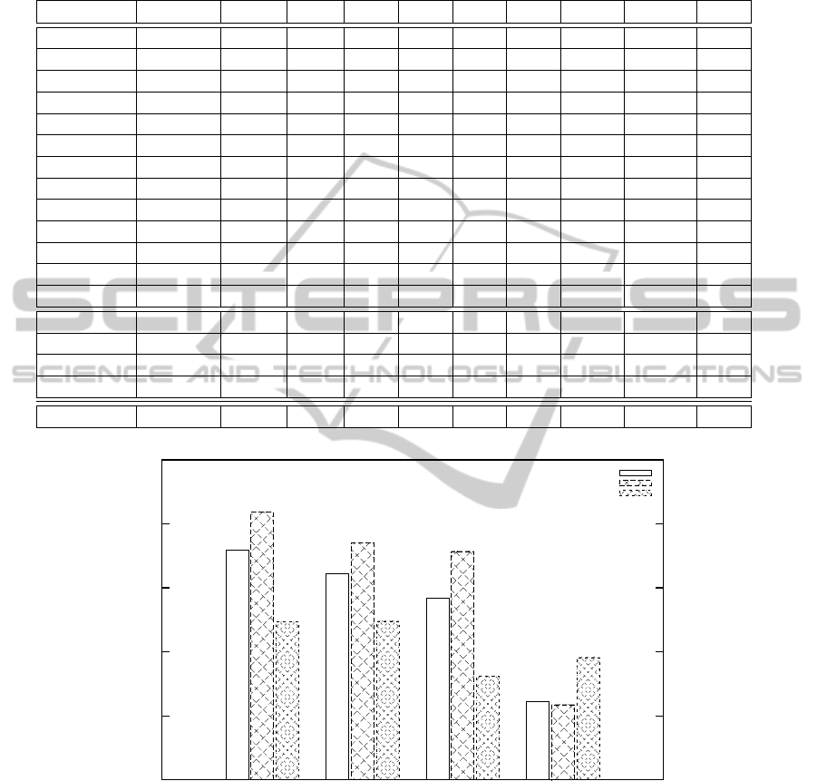
Table 4: Comparison of the feature weighting methods. Compared approaches are Fragment Length Weighted Category
Distribution (FLWCD), T × T, Bi-Normal Separation (BNS), Chi-squared (χ
2
), Pointwise Mutual Information (MI), Infor-
mation Gain (IG), Odds Ratio (OR), Residual IDF (RIDF), Term Frequency (TF), and Term Frequency - Inverse Document
Frequency (TFIDF).
Dataset FLWCD T × T BNS χ
2
MI IG OR RIDF TFIDF TF
Y Q1 0.76 0.76 0.72 0.72 0.76 0.75 0.75 0.75 0.75 0.69
Y Q2 0.76 0.74 0.76 0.77 0.79 0.76 0.75 0.76 0.77 0.72
C Q1 0.50 0.50 0.46 0.44 0.46 0.43 0.46 0.37 0.40 0.43
C Q2 0.70 0.69 0.69 0.60 0.67 0.67 0.69 0.66 0.64 0.55
C2 Q1 0.72 0.68 0.67 0.63 0.66 0.58 0.69 0.62 0.62 0.58
C2 Q2 0.73 0.73 0.74 0.68 0.76 0.75 0.73 0.72 0.69 0.57
C2 Q3 0.71 0.71 0.71 0.68 0.71 0.67 0.69 0.62 0.64 0.58
V Q1 0.79 0.78 0.75 0.70 0.75 0.69 0.80 0.76 0.76 0.65
V Q2 0.68 0.67 0.65 0.63 0.60 0.42 0.67 0.58 0.58 0.60
V Q3 0.79 0.79 0.77 0.70 0.74 0.64 0.76 0.77 0.76 0.70
V Q4 0.75 0.76 0.74 0.72 0.74 0.74 0.74 0.73 0.73 0.71
V Q5 0.70 0.69 0.72 0.68 0.71 0.63 0.71 0.66 0.66 0.63
Avg Mrk 0.72 0.70 0.70 0.66 0.70 0.65 0.70 0.67 0.67 0.62
T M 0.84 0.84 0.76 0.73 0.71 0.80 0.75 0.81 0.80 0.80
T HT 0.81 0.77 0.76 0.73 0.68 0.61 0.77 0.37 0.42 0.48
T RM 0.55 0.46 0.43 0.58 0.36 0.36 0.50 0.21 0.19 0.24
Avg Tw 0.73 0.69 0.64 0.70 0.58 0.59 0.67 0.46 0.47 0.51
Ttl Avg 0.73 0.70 0.67 0.68 0.64 0.62 0.69 0.57 0.57 0.57
0
0.2
0.4
0.6
0.8
1
SVM
TxT
kNN
NB
F-Score
Precision
Recall
Figure 2: Comparison of average F
0.5
-score, Precision and Recall of each classification approach. The average is the average
among all the testsets (instead of test cases). This figure shows where the difference in performance comes from.
ment categorization. In addition, we proposed a novel
feature weighting approach called Fragment Length
Weighted Category Distribution that is designed di-
rectly for short documents by taking the TF=1 chal-
lenge into consideration.
The proposed approach uses Bi-Normal Separa-
tion with inverse average fragment length and word’s
distribution among categories. The experiments sup-
ported our hypothesis that term frequency based
methods struggle when weighting short documents.
In addition, we found that the best performance
among the categorization methods was received using
a Support Vector Machine classifier. When compar-
ing the feature weighting approaches, FLWCD pro-
duced the best results.
In the future we will continue our work on feature
weighting in short documents and utilize the approach
in other relevant domains. We do believe that the pro-
CategorizationofVeryShortDocuments
15

posed approach leaves room for improvement but in
these experimental cases it has produced good results
and shown that it can be used for text categorization
in real world applications.
ACKNOWLEDGEMENTS
The authors wish to thank Taloustutkimus Oy for sup-
porting the work, and Prof. Hannu Toivonen and the
anonymous reviewers for their valuable comments.
REFERENCES
Benevenuto, F., Mango, G., Rodrigues, T., and Almeida,
V. (2010). Detecting spammers on twitter. In CEAS
2010. Seventh annual Collaboration, Electronic messag-
ing, Anti-Abuse and Spam Conference, Redmond, Wash-
ington, USA, July 13 - 14, 2010.
Cai, L. and Hofmann, T. (2003). Text categorization by
boosting automatically extracted concepts. In SIGIR
2003: Proceedings of the 26th Annual International
ACM SIGIR Conference on Research and Development
in Information Retrieval, Toronto, Canada, July 28 - Au-
gust 1, 2003, pages 182–189. ACM.
Clark, K. and Gale, W. (1995). Inverse document frequency
(idf): A measure of deviation from poisson. In Third
Workshop on Very Large Corpora, Massachusetts Insti-
tute of Technology Cambridge, Massachusetts, USA, 30
June 1995, pages 121–130.
Forman, G. (2003). An extensive empirical study of fea-
ture selection metrics for text classification. J Machine
Learning Res, 3:1289–1305.
Forman, G. (2008). Bns feature scaling: an improved rep-
resentation over tf-idf for svm text classification. In Pro-
ceedings of the 17th ACM Conference on Information
and Knowledge Management, CIKM 2008, Napa Valley,
California, USA, October 26-30, 2008, pages 263–270.
ACM.
Irani, D., Webb, S., Pu, C., and Li, K. (2010). Study of
trendstuffing on twitter through text classification. In
CEAS 2010, Seventh annual Collaboration, Electronic
messaging, Anti-Abuse and Spam Conference, Redmond,
Washington, USA, July 13 - 14, 2010.
Joachims, T. (1998). Text categorization with support vec-
tor machines: Learning with many relevant features. In
Machine Learning: ECML-98, 10th European Confer-
ence on Machine Learning, Chemnitz, Germany, April
21-23, 1998, volume 1398 of Lecture Notes in Computer
Science, pages 137–142. Springer.
Joachims, T. (1999). Advances in Kernel Methods - Sup-
port Vector Learning, chapter Making large-Scale SVM
Learning Practical, pages 41–56. MIT Press.
Kibriya, A. M., Frank, E., Pfahringer, B., and Holmes, G.
(2004). Multinomial naive bayes for text categorization
revisited. In AI 2004: Advances in Artificial Intelli-
gence, 17th Australian Joint Conference on Artificial In-
telligence, Cairns, Australia, December 4-6, 2004, vol-
ume 3339 of Lecture Notes in Computer Science, pages
488–499. Springer.
Krishnakumar, A. (2006). Text categorization build-
ing a knn classifier for the reuters-21578 collec-
tion. http://citeseerx.ist.psu.edu/viewdoc/-summary?
doi=10.1.1.135.9946.
Mladenic, D. and Grobelnik, M. (1999). Feature selec-
tion for unbalanced class distribution and naive bayes.
In Proceedings of the Sixteenth International Conference
on Machine Learning (ICML 1999), Bled, Slovenia, June
27 - 30, 1999, pages 258–267. Morgan Kaufmann.
Pak, A. and Paroubek, P. (2010). Twitter as a corpus for
sentiment analysis and opinion mining. In Proceedings
of the International Conference on Language Resources
and Evaluation, LREC 2010, Valletta, Malta, 17-23 May
2010. European Language Resources Association.
Phan, X. H., Nguyen, M. L., and Horiguchi, S. (2008).
Learning to classify short and sparse text & web with
hidden topics from large-scale data collections. In Pro-
ceedings of the 17th International Conference on World
Wide Web, WWW 2008, Beijing, China, April 21-25,
2008, pages 91–100. ACM.
Rennie, J. D., Shih, L., Teevan, J., and Karger, D. R. (2003).
Tackling the poor assumptions of naive bayes text clas-
sifiers. In Machine Learning, Proceedings of the Twen-
tieth International Conference (ICML 2003), August 21-
24, 2003, Washington, DC, USA, pages 616–623. AAAI
Press.
Rennie, J. D. M. and Jaakkola, T. (2005). Using term infor-
mativeness for named entity detection. In SIGIR 2005:
Proceedings of the 28th Annual International ACM SI-
GIR Conference on Research and Development in Infor-
mation Retrieval, Salvador, Brazil, August 15-19, 2005,
pages 353–360. ACM.
Ritter, A., Cherry, C., and Dolan, B. (2010). Unsupervised
modeling of twitter conversations. In Human Language
Technologies: Conference of the North American Chap-
ter of the Association of Computational Linguistics, Pro-
ceedings, Los Angeles, California, USA, June 2-4, 2010,
pages 172–180. The Association for Computational Lin-
guistics.
Salton, G. and Buckley, C. (1988). Term-weighting ap-
proaches in automatic text retrieval. Inf Process Manage,
24(5):513–523.
Timonen, M., Silvonen, P., and Kasari, M. (2011). Classifi-
cation of short documents to categorize consumer opin-
ions. In Advanced Data Mining and Applications - 7th
International Conference, ADMA 2011, Beijing, China,
December 17-19, 2011. Online Proceedings.
Yang, Y. (1999). An evaluation of statistical approaches to
text categorization. Inf. Retr., 1(1-2):69–90.
Yang, Y. and Liu, X. (1999). A re-examination of text
categorization methods. In SIGIR ’99: Proceedings of
the 22nd Annual International ACM SIGIR Conference
on Research and Development in Information Retrieval,
Berkeley, CA, USA, August 15-19, 1999, pages 42–49.
ACM.
Yang, Y. and Pedersen, J. (1997). Feature selection in sta-
tistical learning of text categorization. In Proceedings
of the Fourteenth International Conference on Machine
Learning (ICML 1997), Nashville, Tennessee, USA, July
8-12, 1997, pages 412–420.
KDIR2012-InternationalConferenceonKnowledgeDiscoveryandInformationRetrieval
16
