
Geometric Image of Neurodynamics
Germano Resconi
1
and Robert Kozma
2
1
Dept. of Mathematics and Physics, Catholic University Brescia, Brescia, I-25121, Italy
2
Dept. of Mathematical Science, Computational Neurodynamic Laboratory, University of Memphis,
Memphis, TN 38152, U.S.A.
Keywords: Conceptual Intention, Material Intention, Electrical Circuit, Memristor, Neuromorphic Computing,
Geodesic Conductance Matrix, Impedance Matrix, Software, Hardware, Digital Computer,
Multidimensional Space of Currents, Charges and Voltages.
Abstract: We know that the brain is composed of simple neural units given by dendrites, soma, and axons. Every
neural unit can be modelled by electrical circuits with capacitors and adaptive resistors. To study the neural
dynamic we use special Ordinary Differential Equations (ODE) whose solutions give us the behaviour or
trajectory of the neural states in time. The problem with ODE is in the definition of the parameters and in
the complexity of the solutions that in many cases cannot be found. The key elements that we use are the
multidimensional vector spaces of the electrical charges, currents and voltages. So currents and voltages are
geometric references for states in the central neural system (CNS). Any neuro –biological architecture can
be modelled by an adaptive electrical circuit or neuromorphic network that relates voltage with current by
conductance matrix or on the contrary by impedance matrix. Given a straight line with a change of reference
we reshape the straight line in a geodetic and in a new form for the distance. The change of the reference
transforms a set of variables into another so this transformation is similar to a statement in the digital
computer that we associate to the software. Every change of variables can be reproduced by a similar
change of voltages (currents) into currents (voltages) by conductance (impedance) matrix. We use the CNS
as a material support or hardware in the digital computer to realise the wanted transformation. In conclusion
geometry fuses the digital computer structure with neuromorphic computing to give efficient computation
where conceptual intention is the change of the reference space , while material intention is given by the
neurodynamical processes modelled by the change of the electrical charge space where we define the metric
geometry and distance.
1 INTRODUCTION
This work studies a possible mathematical
formulation of intentional brain dynamics following
Freeman’s half century-long dynamic systems
approach (Freeman, 1975; 2007); (Kozma, 2008)
We consider the electrical behaviour of the brain. In
1980 an artificial neural network was built that
works but has high precision components, slow
unstable learning, it is non adaptive and needs an
external control. Now we want low precision
components, fast stable learning, adapt to
environment and autonomous. How can we get this?
We can make dynamical components, add feedback
(positive & negative) and close the loop with the
outside world. The ordinary differential equations or
ODEs to control the neural dynamic are a stiff and
nonlinear system. Why not just program this on a
computer? We know that stiff and nonlinear
dynamical systems are inefficient on a digital
computer. An example is the IBM Blue Gene project
with 4096 CPUs and 1000 Terabytes RAM, which,
to simulate the Mouse cortex uses 8 10
6
neurons, 2
10
10
synapses 109 Hz, 40 Kilowatts and digital. The
brain uses 10
10
neurons, 10
14
synapses 10 Hz and 20
watts analog system which is more efficient than
digital by many orders of magnitude.
(Snider, 2008) suggests to use analog electrical
circuit denoted CrossNet or neuromorphic computing
with memristor to solve the problem of the neural
computation. Let’s recall that for Turing the physical
devise is not computable by a Turing machine, which
is the theoretical version of the digital computer.
(Carved, 1990) suggests that the physics or analog
computer is more efficient to solve the neural network
problem. In fact, for analog system we do not have
457
Resconi G. and Kozma R..
Geometric Image of Neurodynamics.
DOI: 10.5220/0004110204570465
In Proceedings of the 4th International Joint Conference on Computational Intelligence (NCTA-2012), pages 457-465
ISBN: 978-989-8565-33-4
Copyright
c
2012 SCITEPRESS (Science and Technology Publications, Lda.)
algorithms to program the neurons. Rather, the digital
program is substituted by the dynamics in non
Euclidean space. We can program the CrossNet
(Takashi Kohno, 2008), (Rinzel, 1998) electrical
system as it was used by Snider to compute the
parameters useful to generate the desired trajectories
to solve problems. Geometric and physical
description of the intentionality (Freeman, 1975) is
beyond any algorithmic or digital computation. To
clarify better the new computation paradigm, we can
refer the following principle: “Animals and humans
use their finite brains to comprehend and adapt to
infinitely complex environment.” (Kozma, 2008) We
show that this adaptive system has a geometric
interpretation that gives us the possibility to
implement the required parameters in ODE to achieve
the desired behaviours. The geometric interpretation
uses three main spaces. One is the current
multidimensional space, the other is the electrical
charge multidimensional space and the last is the
voltage space (Resconi, 2007; 2009). In (Mandzel,
1999) we can found geometric method to study
human motor control.
2 GEOMETRY AND
ELECTRICAL CIRCUITS
Because the brain is a complex electrical circuit with
capacity and resistors, a network of neurons or an
electronic network is a general transformation or
MIMO from many voltages in inputs to many
currents in output
( , ,..., )
1
11 2
( , ,..., )
2
212
...
( , ,..., )
12
ifvv v
p
ifvv v
p
ifvv v
n
np
(1)
where the currents are vectors in a n-dimensional
space of the currents and the voltages are vectors in
a p-dimensional space. In figure 1 we show as
Figure 1: Vector of current in the current space.
example the three dimensional current space.
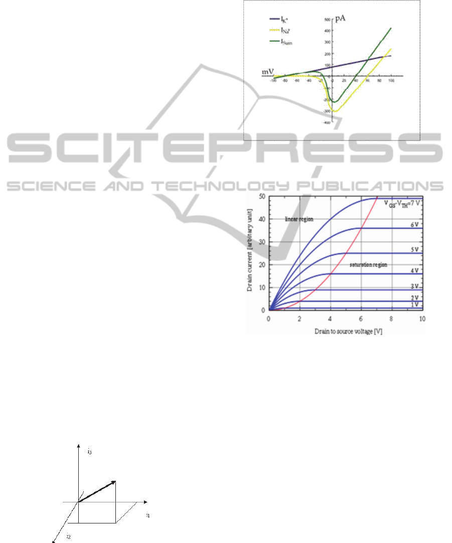
For one dimension the (1) is written in this form
()ifv
that in electronics is denoted characteristic
function. In Figures 2 and 3 we show two different
cases for (1) in one dimension.
Figure 2: An approximation of the potassium and sodium
ion components of a so-called "whole cell" I–V curve of a
neuron.
Figure 3: MOSFET drain current vs. drain-to-source
voltage for several values of the overdrive voltage, V
GS
-
V
th
; the boundary between linear (Ohmic) and saturation
(active) modes is indicated by the upward curving
parabola.
The instrument to match intentionality with the
electrical circuit is the metric geometry of the brain
state space or electrical charge space. The metric
geometry in the state space can be obtained by the
instantaneous electrical power p in the current space
or in voltage space as we show in equation (2). For
the linear form of the (1) we have the expression of
the power.
IJCCI2012-InternationalJointConferenceonComputationalIntelligence
458

ds
2
( ) = power = i v + i v +,.....,+i v
11 22 nn
dt
for
CC...C
iv
1,1 1,2 1,n
11
CC ...C
iv
22
2,1 2,2 2,n
=
... ...
... ... ... ..
iv
CC ...C
nn
n,1 n,2 n,n
we have
2
power = C v +,..,+2 C v v + 2C v v + .
1,1 1 1,2 1 2 1,3 1 3
.
=C vv=Z ii
α,βα,β
αα
α,βα,β
(
2
)
2
dq
dq
Z
α,β
dt dt
α,β
and
ds Z dq
α,β
α,β
ds
dt
dq
(2)
(3)
Where
,
C
and
,
Z
are the conductance matrix
and the impedance matrix, v are the voltages , i are
the currents and q are the charges. For example,
given the electrical circuit.
Figure 4: Simple electrical circuit with three generators
V1, V2, V3.
For the Kirchhoff current and voltage laws and
for Ohm’s law we have for the electrical circuit in
Figure 4 the following system of equations.
12 1
32 2
213
111 22
23322
VV E
VV E
iii
ERiRi
ERiRi
whose solution is
()
231 2
1
12 13 23
()
3
2
12 13 23
()
2
3
12 13 23
32
31
12
3
12 13
123 1
RRV R
i
RR RR R R
RRV R
i
RR RR R R
RRV R
i
RR RR R R
RV V
RV V
RV V
(4)
For the vector space of currents and voltages the
Kirchhoff current and voltage laws and Ohm’s laws
can be represented in this vector form
1
1
13
3
3
1
12
1
2
32
2
3
00
1
00
2
00
3
i
i
10
1
i
i11 i+i
2
i
01
i
i
3
T
10
V
E
11
V
E
01
Ri
11
Ri
22
Ri
33
V
V
V
V
V
V
V
V
where the solutions can be written in an operational
way in this form
GeometricImageofNeurodynamics
459

1
2
00
1
1
00
2
3
00
3
1
3
00
1
1
(( 0 0 )
2
00
3
i
T
v
10
1
E
11 v
2
E
01
v
3
T
R
10 10
i
11 R 11
i
01 01
R
i
10
1
i
i11
2
i
01
i
3
T
R
10 10 10 10
i 11 11 R 11 11
01 01 01 01
R
) v
v
vv
v
T
1
2
3
00
1
1
(00)
2
00
3
23 3 2
1
()
3131 121332
2112
iCv
TT
R
10 10 10 10
C 11 11 R 11 11
01 01 01 01
R
RR R R
CRRRRRRRRRR
RRRR
So for
where C is the conductance matrix for which
1,1 1,2 1,3
11
22,12,22,32
33
3,1 3,2 3,3
11,111,221,23
22,112,222,33
33,113,223,33
CC C
iv
iCCCv
iv
CC C
or
iCvCv Cv
iCvCvCv
iCvCvCv
For relation (1) we can compute the dynamical
conductance
11 1
...
12
...
1,1 1,1 1,1
22 2
...
...
1,1 1,1 1,1
12
... ... ... ...
... ... ... ...
...
1,1 1,1 1,1
...
12
ii i
vv v
p
CC C
ii i
CC C
C
vv v
p
CC C
ii i
nn n
vv v
p
(5)
C is the dynamical conductance which is the
function of the voltages
(, ,..., )
12
CCvv v
p
The instantaneous power is
p
ower = i v = C v v where
j
j
j,k k
j.k
j
-1 -1
i=Cv,v=C i=Zi,Z=C
j
and
11
()()
,
,
TT
Cvv vCv CiCCi
jk
kj
jk
1
,
,
TT
iC i iZi Z ii
jk
kj
jk
(6)
In the next chapter we show how it is possible by the
geodesic in the charge space to generate the ordinary
differential equation (ODE) that controls the
dynamics of the neural network and of the electrical
circuit.
3 SIMPLE ELECTRICAL
CIRCUIT AND GEODESIC
Given the trivial electrical circuit
V
3
V
4
E
i
1
V
1
V
2
R
Figure 5: Simple electrical circuit with one generator E
and one resistor R.
We compute the power p that is dissipated by the
resistance R. We define the infinitesimal distance ds
in this way:
22
= ( )
dq
power Ri R
dt
ds
dt
We know that in the electrical circuit the currents
flow in the circuit in such a way to dissipate the
minimum power. The geodesic line in the one
IJCCI2012-InternationalJointConferenceonComputationalIntelligence
460

dimension current space i is the trajectory in time.
For the minimum dissipation of the power or cost C,
we have
2
() 0
dq
Cds Wdt R dt
dt
We can compute the behavior of the charges for
which we have the geodesic condition of the
minimum cost. We know that this problem can be
solved by the Euler Lagrange (Izrail, 1963)
differential equations or ODE (ordinary differential
equation)
22
() ()
0
dq dq
RR
d
dt dt
dq
dt q
dt
When R is independent of the charges then R has no
memory , so the previous equation can be written as
follows
()
2
0 , ( ) ,
2
dq
d
dq dq E
dt
qt at b i a
dt dt R
dt
The geodesic is a straight line in the space of the
charge. In Figure 6 we show the behaviour of the
geodesic in the charge space and the current space as
derivatives of the electrical charges
Figure 6: Charge space and derivatives in time of charges
or currents.
4 DIGITAL AND NEURAL
COMPUTING
To stress the difference between digital computer
and geometric map of the brain we refer the
interesting discussion of (Carver, 1990) where are
present all the main ideas that we use and improve in
this paper. Biological solutions in formation
processing systems operate on completely different
principles from those with which most engineers are
familiar. For many problems, particularly those in
which the input data are ill-conditioned and the
computation can be specified in a relative manner,
biological solutions are many orders of magnitude
more effective than those we have been able to
implement using digital methods. This advantage
can be attributed principally to the use of elementary
physical phenomena as computational primitives,
and to the representation of information by the
relative values of analog signals, rather than by the
absolute values of digital signals. A typical
microprocessor does about 10 million operations and
uses about 1 W. In round numbers, it costs about
l0
-7
J to do one operation, the way we do it today, on
a single chip. If we go off the chip to the box level, a
whole computer uses about 10
-5
J /operation. A
whole computer is thus about two orders of
magnitude less efficient than is a single chip. Back
in the late 1960's we analyzed what would limit the
electronic device technology as we know it; those
calculations have held up quite well to the present.
The standard integrated circuit fabrication processes
available today allow us to build transistors that
have minimum dimensions of about 1 ( 10
-6
m).
By ten years from now, we will have reduced these
dimensions by another factor of 10, and we will be
getting close to the fundamental physical limits: if
we make the devices any smaller, they will stop
working. It is conceivable that a whole new class of
devices will be invented that are not subject to the
same limitations. But certainly the ones we have
thought of up to now-including the superconducting
ones-will not make our circuits more than about two
orders of magnitude more dense than those we have
today. The factor of 100 in density translates rather
directly into a similar factor in computation
efficiency. So the ultimate silicon technology that
we can envision today will dissipate on the order of
10
-9
J of energy for each operation at the single chip
level, and will consume a factor of 100-1000 more
energy at the box level. We can compare these
numbers to the energy requirements of computing in
the brain. There are about 10
16
synapases in the
brain. A nerve pulse arrives at each synapse about
ten times, on average. So in rough numbers, the
brain accomplishes 10
16
complex operations. The
power dissipation of the brain is a few watts, so each
operation costs only 10
-16
J. The brain is a factor of 1
billion more efficient than our present digital
technology, and a factor of 10 million more efficient
than the best digital technology that we can imagine.
From the first integrated circuit in 1959 until
GeometricImageofNeurodynamics
461

today, the cost of computation has improved by a
factor about 1 million. We can count on an
additional factor of 100 before fundamental
limitations are encountered. At that point, a state-of-
the-art digital system will still require 10MW to
process information at the rate that it is processed by
a single human brain. The unavoidable conclusion,
which (Carver, 1990) reached about ten years ago, is
that we have something fundamental to learn from
the brain about a new and much more effective form
of computation. Even the simplest brains of the
simplest animals are awesome computational
instruments. They do computations we do not know
how to do, in ways we do not understand. We might
think that this big disparity in the effectiveness of
computation has to do with the fact that, down at the
device level, the nerve membrane is actually
working with single molecules. Perhaps
manipulating single molecules is fundamentally
more efficient than is using the continuum physics
with which we build transistors. If that conjecture
were true, we would have no hope that our silicon
technology would ever compete with the nervous
system. In fact, however, the conjecture is false.
Nerve membranes use populations of channels,
rather than individual channels, to change their
conductances, in much the same way that transistors
use populations of electrons rather than single
electrons. It is certainly true that a single channel
can exhibit much more complex behaviors than can
a single electron in the active region of a transistor,
but these channels are used in large populations, not
in isolation (Carver, 1990). We can compare the two
technologies by asking how much energy is
dissipated in charging up the gate of a transistor
from a 0 to a 1. We might imagine that a transistor
would compute a function that is loosely comparable
to synaptic operation. In today’s technology, it takes
about 10
-13
j to charge up the gate of a single
minimum-size transistor.
In ten years, the number
will be about 10
-15
j within
shooting range of the
kind of efficiency realized by nervous
systems. So
the disparity between the efficiency of computation
in the nervous system and that in a computer is
primarily attributable not to the individual device
requirements,/operation. A whole computer is thus
about two orders of magnitude less efficient than is a
single chip. The disparity between the efficiency of
computation
in the nervous system and that in a
computer is
primarily attributable not to the
individual device requirements,
but rather to the way the devices are used in the
system.
Where did all the energy go? There is a factor of 1
million unaccounted for between what it costs to
make a transistor work and what is required to do an
operation the way we do it in a digital computer.
There are two primary causes of energy waste in the
digital systems we build today.
1) We lose a factor of about 100 because, the way
we build digital hardware, the capacitance of the
gate is only a very small fraction of capacitance of
the node. The node is mostly wire, so we spend most
of our energy charging up the wires and not the gate.
2) We use far more than one transistor to do an
operation; in a typical implementation, we switch
about 10 000 transistors to do one operation. So
altogether it costs 1 million times as much energy to
make what we call an operation in a digital machine
as it costs to operate a single transistor. (Carver,
1990) does not believe that there is any magic in the
nervous system, that there is a mysterious fluid in
there that is not defined, some phenomenon that is
orders of magnitude more effective than anything we
can ever imagine.
There is nothing that is done in the nervous
system that we cannot emulate with electronics if
we understand the principles of neural
information processing by suitable conceptual or
software transformations in general reference
(geometry ).
We can starts by letting the device physics define
elementary operations. These functions provide a
rich set of computational primitives, each a direct
result of fundamental physical principles. They are
not the operations out of which we are accustomed
to building computers, but in many ways, they are
much more interesting. They are more interesting
than AND and OR. They are more interesting than
multiplication and addition. But they are very
different. (Carver,1990) tries to fight them, to turn
them into something with which we are familiar, he
thinks to end up making a mess. We show in this
paper that this is not true. In fact (Carver,1990)
forgot that the new operations must be oriented to a
specific goal or intension. Now we are in agreement
with and his neuromorphic network but we add a
new dimension to the electrical system by the
geometry in multidimensional space of charges to
mimic the wanted transformation in the
multidimensional space of the states.
So the real trick is to invent a vector
representation of the electrical charges that
takes advantage of the inherent capabilities of
the medium, such as the abilities to mimic the
wanted transformation. These are powerful
primitives. In conclusion we use the nervous
IJCCI2012-InternationalJointConferenceonComputationalIntelligence
462

system as an instrument to simulate system-
design strategy oriented to the wanted goal or
intentionality.
5 GEOMETRY AND
CONCEPTUAL PART IN
NEURAL NETWORK
Now the electrical power gives us the material
aspect of intentionality. The other part of
intentionality is the conceptual one which is given
by the wanted transformation
( , ,... )
1112
( , ,... )
2212
...
( , ,... )
12
yyxxx
p
yyxxx
p
yyxxx
qq p
(7)
where
( , ,..., )
12
x
xx
p
are the initial variables and
(y , y ,..., y )
n
12
are the wanted final variables. Now
with the transformation (7) we can write the local
linear equation
11 1
....
11 2
12
22 2
....
212
12
...
....
12
12
yy y
dy dx dx dx
p
xx x
p
yy y
dy dx dx dx
p
xx x
p
yy y
qq q
dy dx dx dx
qp
xx x
p
So we have
222 2 2
11
..... ( .... )
1
12
1
22
22
( .... ) ... ( .... )
,
11
,
11
yy
ds dy dy dy dx dx
p
q
xx
p
yy
yy
qq
dx dx dx dx G dx dx
jk
pp
j
k
xx xx
jk
pp
12
...
11 1
12
...
22 2
,
... ... ... ...
12
y
yy
q
xx x
y
yy
q
xx x
GG
jk
yy
xx
pp
12
...
11 1
12
...
22 2
... ... ... ...
12
... ...
T
y
yy
q
xx x
y
yy
q
T
xx x
J
J
yy
yy
qq
xxx x
ppp p
(8a)
The identity between the geometric metric G with
the electrical circuit metric Z is the fundamental
equation that connects conceptual transformation (7)
with physical transformation (1).
where the distance is in the charge space
,,
GZ
ij ij
With the fundamental equation we can compute the
parameters of the distance as the square of the power
in the electrical circuit. The square of the power is a
non Euclidean distance in the state space of the
electrical circuit that simulates the non Euclidean
space of the classical geometry.
Example:
Let’s begin with an example. When the conceptual
intention moves on a sphere given by simple
equation
2222
123
yyy
r
Figure 7: sphere where the green, red and blue lineas are
geodetic.
we have the transformations ( conceptual intention )
sin( ) cos( )
1
sin( ) sin( )
2
cos( )
3
xr
xr
xr
Let’s compute the geodesic in the space (x
1
, x
2
, x
3
)
So we have
2222
3
12
(,)()( )( )]
22
11 2 2
()( )
dx
dx dx
ds
dt dt dt
dx dx dx dx
dd d d
d dt d dt d dt d dt
(8b)
22 222 2
33
()()sin()()
dx dx
dd d d
rr
d dt d dt dt dt
for the fundamental equation G
i,j
= Z
i,j
we have
2
0
22
0sin()
r
Z
r
GeometricImageofNeurodynamics
463
The current is
1
2
,
d
i
22 2 2 2
dt
power = r i + r sin (q )i
112
id
dt
(9)
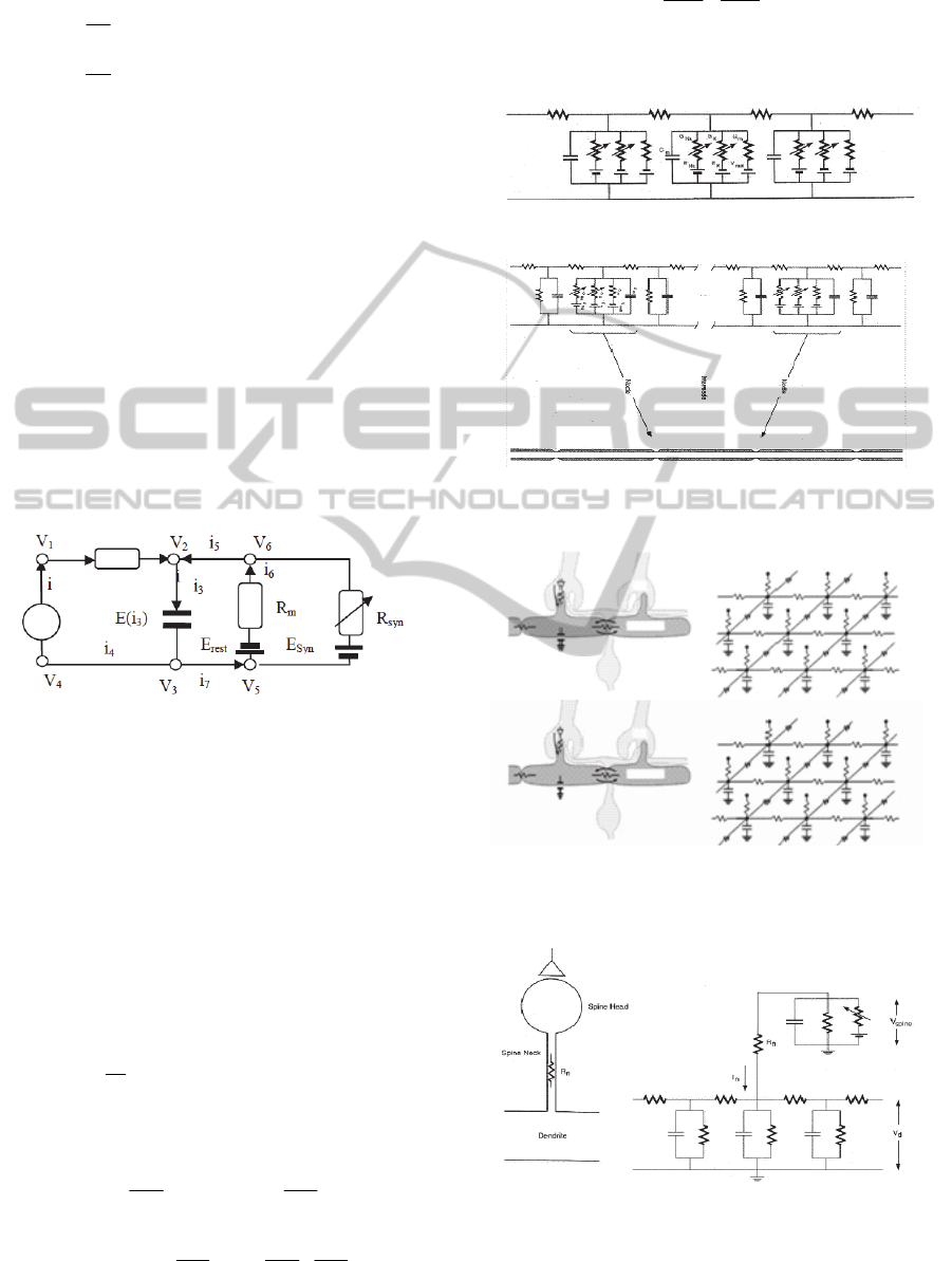
6 NEURAL SYSTEM AS A
COMPLEX ELECTRICAL
CIRCUIT (FIGURE 12)
In opposition to actual digital sequential computers
where computations are carried out by a single
complex processor there are Cellular Neural/Non-
linear Networks (CNN) (Torralba, 1999) which are
analog parallel machines with a high number of
simple processors, which are disposed in a regular
array, and each processor is connected to the other
processors in a reduced neighborhood. One of these
analog processors is represented by the electrical
activity of the synapse given by the electrical circuit
Figure 8: Electrical circuit of the synapse.
The impedance matrix is
31 0
13
02
R
ins
ZRR
mm
RRR
msynm
The geodesic trajectory of the synapse activity is
controlled by the relation
power = i
T
Z i
where Z is the impedance matrix in the currents
space. In an extensive form we have
222
() ( 3) ( 3)
5
2
2
(2)+ 22
55
82 8
22
(3)()(3)()
2
( 2)( ) + 2( )( )
5
2
85
2
d
s
power R i R i
m
ins
dt
RR i ii Rii
msys m
dq
dq
RR
m
ins
dt dt
dq dq
dq
RR
msys
dt dt dt
2( )( )
58
dq dq
R
m
dt dt
(10)
We will show examples of simulation of a neuronal
network by an equivalent electrical circuit.
Figure 9: Example of axon and electrical circuit.
Figure 10: Axon with myelin and equivalent electrical
circuit.
Figure 11: On the left there are the cones, the orizontal
neurons and bipolar neurons. On the right there are the
neuromorphic diagram or equivalent electrical circuit.
Figure 12: Complex electrical circuit of neural network
system.
For more complex neural networks, we can
IJCCI2012-InternationalJointConferenceonComputationalIntelligence
464

derive the corresponding geodesics in a similar
fashion. For example, we could consider have the
electrical representation of a neural network as
shown in Figure 12.
7 CONCLUSIONS
With the neural network we can simulate the
geodesic movement for any transformation of
reference. For a given transformation of reference,
we can build the associate geodesic, which allows to
implement the transformation of reference in the
neural network. The neural network as analog
computer gives the solution of the ODE of the
geodesic inside the wanted reference. The Freeman
K set (Freeman, 1975) is the ODE of the geodesic
that is the best trajectory in the space of the
electrical charges. (Freeman, 1975) introduced the
concept of intentionality, which can be recognized
and studied in its manifestations of goal-directed
behavior. Intention is interpreted as, respectively, an
attribute of mental representations, the expression of
motivations and biological driver. The mental
representation is the conceptual part (software) of
the intention, the biological driver is the material
part (hardware) of the intention.
In this paper we showed that any part of the brain
can be represented by a complex electrical circuit.
Intention has two different parts: the one is the
conceptual part given by wanted transformation of
the brain states. In the new reference the deformed
straight line, geodesic, is the minimum distance
between two points in the state space as in the
classical straight line. The other part is the material
part of the intention. In fact because any part of the
brain can be modelled by an electrical circuit, and
because the transformations between the voltages
and currents give us the change of the reference ,the
real transformation in the brain states is the material
part of the intention. The conceptual parameters and
the material parameters G (conductance C or
impedance Z) must be equal. When the two parts are
equal we have defined the central nervous system
CNS dynamics in agreement with the wanted
transformation in the conceptual space. The CNS
realizes in the material world the wanted
transformation. We define a task in the conceptual
domain and we can implement the task in the
material neural network parametric structures. In
comparison with the traditional digital computer the
conceptual part of intention is the software and the
material part of intention is the hardware. The
difference in the geometry of intention theory and
digital computer is in the representation of the
software and hardware. In the digital computer we
have logic statements for the software and logic
gates for the hardware. In the geometry of the
intention we have geometric changes of the
references in the multidimensional space as software
and neural network as hardware.
REFERENCES
Walter J. Freeman 1975 Mass Action in The Nervous
System. Academic Press, New York San Francisco
London.
R. Kozma W. J. Freeman, (2008 ) “Intermittent spatial –
temporal desynchronization and sequenced synchrony
in ECoG signal“ Interdisciplinary J. Chaos
18.037131.
Freeman, W. J. A 2007 pseudo-equilibrium
thermodynamic model of information processing in
nonlinear brain dynamics. Neural Networks (2008),
doi:10.1016/ j.neunet..12.011.
Takashi Kohno and Kazuyuki Aihara, 2008) A Design
Method for Analog and Digital Silicon Neurons
Mathematical-Model-Based Method-, AIP Conference
Proceedings, Vol. 1028, pp. 113–128.
J. Rinzel and B. Ermentrout, 1998 “Analysis of Neural
Excitability and Oscillations,” in “Methods in Neural
Modeling”, ed. C. Koch and I. Segev, pp. 251–291,
MIT Press, 1998.
Germano Resconi 2007, Modelling Fuzzy Cognitive Map
by Electrical and Chemical Equivalent Circuits Joint
Conference Information Science July8-24 Salt lake
City Center USA.
Germano Resconi, Vason P.Srini 2009 Electrical Circuit
As A Morphogenetic System, GEST International
Transactions on Computer Science and Engineering
volume 53, Number 1 pag.47-92.
Amir A. Mandzel, Tomar Flach 1999 Geometric Methods
in the study of human motor control. Cognitive Studies
6 (3) p.309 – 321.
Greg S. Snider 2008 Hewlett packard Laboratory,
Berkeley conference on memristors.
Carver Mead 1990, Neuromoprhic Electronic Systems,
Proceeding of the IEEE vol.78 No.10
Antonio B. Torralba 1999, Analogue Architectures for
Vision Cellular Neural Networks and Neuromorphic
Circuits, Doctorat thesis, Institute national
Polytechnique Grenoble, Laboratory of Images and
Signals.
Izrail Moiseevich Gelfand 1963. Calculus of Variations.
Dover.
GeometricImageofNeurodynamics
465
