
Illustrating the Difficulties of Zimmermann Method for Solving the
Fuzzy Linear Programming by the Geometric Approach
M. R. Safi and A. Razmjoo
Department of Mathematics, Semnan University, Semnan, Iran
Keywords: Fuzzy Linear Programming, Zimmermann Method, The Geometric Method.
Abstract: In this paper we first recall Zimmermann method and the Geometric approach for solving fuzzy linear
programming problem. We show, by the geometric approach, Zimmerman method has some difficulties.
Numerical examples are provided for illustrating the difficulties. Finally, the IZM algorithm for improving
Zimmermann method is recalled.
1 INTRODUCTION
Following "Decision Making in Fuzzy Environment"
proposed by (Bellman and Zadeh, 1970) and "On
Fuzzy Mathematical Programming" proposed by
(Tanaka et al., 1974), Zimmermann, (1976) first
introduced FLP as a conventional LP.
Since then, FLP has been developed in a number
of directions with many wide applications. Among
the others, the approach of (Verdegay, 1982) and
(Chanas, 1983) which presents a parametric
programming method for solving FLP, is the most
often used. Guu and Wu (1999) developed a two-
phase approach for solving the problem, which
concentrates on the fuzzy efficiency of solutions. Safi
et al., (2007) showed some difficulties in ZM by
algebraic approach. They proposed an algorithm
(IZM algorithm), that eliminates these difficulties.
The majority of studies for handling FLP
problems focus on developing different algebraic
methods. Safi et al., (2007) used the fuzzy geometry
proposed by (Rosenfeld, 1994) and presented a
geometric approach for solving FLP problems.
In this note we illustrate the difficulties of
Zimmermann method (ZM) by the geometric
approach.
2 THE ZIMMERMANN METHOD
Consider the following general form of the FLP
problem:
(2.1)
..
~
,
,…,
0
where, and
~
denote the relaxed or fuzzy
versions of the ordinary max and symbols,
respectively. For representing the fuzzy goal, let us
assume that the objective function must be
essentially greater than or equal to an aspiration
level
that has been chosen by the decision maker
(DM). Then we consider the following problem:
,…,
(2.2)
..
~
~
,1,…,
0
The above fuzzy inequalities can be interpreted as
the fuzzy subsets
,0,1,…, of
such that
,
, 0, 0,1,…,, and
0
1
0
1
0
00 0
1
0
00
1
1
( ) 1 1, 2,...,
0,
n
jj
j
n
jj
n
j
jj
j
n
jj
j
cx
cx
cx
cx
if b
b
Cifbpbim
p
if b p
x
(2.3)
435
R. Safi M. and Razmjoo A..
Illustrating the Difficulties of Zimmermann Method for Solving the Fuzzy Linear Programming by the Geometric Approach.
DOI: 10.5220/0004114604350438
In Proceedings of the 4th International Joint Conference on Computational Intelligence (FCTA-2012), pages 435-438
ISBN: 978-989-8565-33-4
Copyright
c
2012 SCITEPRESS (Science and Technology Publications, Lda.)

1
1
1
1
1
() 1 1,2,...,
0,
n
ij j
j
n
ij j
n
j
iijj
j
n
ij j
j
i
i
i
i
i
i
i
i
ax
ax
ax
ax
if b
b
Cifbbpim
p
if b p
x
(2.4)
where
0
p
and
i
p
, i = 1,2,…m are positive constants
subjectively assigned by the DM expressing the
limitation of admissible violation for the fuzzy goal
and the ith fuzzy constraint, respectively. In order to
find the best decision for Problem (2.2)
Zimmermann solves the following problem
00
1
1
max
.. (1 )
(1 ) 1 2, m
0, 1,..., , [0,1].
n
jj
g
n
ij j
j
j
ii
cx
ax
λ
st b p
bpi ,,
xjn
(2.5)
3 THE GEOMETRIC APPROACH
Safi et al., (2007) studied FLP from a geometric
viewpoint. In this section we recall some definitions
and theorems from the geometric approach.
3.1 Fuzzy Geometric Preliminaries
Definition 3.1.1. (Rosenfeld, 1994): A fuzzy subset
C
~
of the plane is called a fuzzy half plane in
direction θif the value of its membership function,
)(
~
θθ
,yxC
, depends only on
θ
x
. In this case, the
membership function should be a monotonically
non-decreasing function.
Theorem 3.1.2. (Safi et al., 2007): Let
be a fuzzy
subset of the plane such that its membership function
in the
, coordinate system is in the form of
Equations (2.3) or (2.4) for
2.Then there exists
a direction
such that
is a fuzzy half plane in this
direction.
Definition 3.1.3. (Rosenfeld, 1994): Let
n
C,...,C,C
~
~
~
21
be fuzzy half planes in directions
n
,...,θ,θθ
21
, respectively. Then
i
n
i
CS
~~
1
is called
a fuzzy polygon
.
Theorem 3.1.4. (Rosenfeld, 1994): If
S
~
is a fuzzy
polygon then
α
S
~
is a crisp polygon for all
.,α ]10[
3.2 Feasibility and Optimality
The following definitions and theorems are from
Safi et al., (2007).
Definition 3.2.1. Consider FLP problem (2.2).
⋂
is called the fuzzy feasible space,
and,
∩
is called the fuzzy decision space.
Here we use the min-operator for intersection.
Definition 3.2.2.A point ∈
is called a -feasible
point of
.
~
S
if
λS )(
~
x
.
Theorem 3.2.3.Every convex combination oftwo λ-
feasible points of
.
~
S
is again a λ-feasible point of
.
~
S
Definition 3.2.4. For
A
~
, set
}.
~
|sup{
*
α
Aαα
Then
*
α
A
~
is called the nonempty supremum cut
(NSC) of the fuzzy set
A
~
and denoted by NSC(
A
~
).
Definition 3.2.5. Let
D
~
be the fuzzy decision space
for the problem (2.1). For
D
~
,
*
α
DD
~
)
~
NSC(
is
called the set of optimal solutions with the optimal
value
*
α
. If
D
~
, we say that the problem does
not have any optimal solution.
Safi, et.al (2007) discussed the optimal solution and
the optimal objective value in Definition 3.2.5 which
are completely consistent with those in ZM.
4 ILLUSTRATING THE
DIFFICULTIES
Safi et al., (2007) has investigated some difficulties
in ZM from the algebraic viewpoint. In this section
we study the difficulties by means of the geometric
approach.
Example 4.1. Consider the following problem:
12
12
12
12
12
max
.. 2 10
~
23
~
212
~
,0.
zx x
st x x
xx
xx
xx
(4.1)
Let
,3
0
b
3,3,2,1
321
pppp
. The
Zimmermann algebraic method solves the associated
problem (2.5) and obtains the alternative optimal
solutions:
)0,3(
*
A
x
,
)3,0(
*
B
x
,
)6.4,8.0(
*
C
x
,
)0,6(
*
D
x
and
)6667.2,6667.4(
*
E
x
with
∗
1.The geometric approach provides Figures 4-1
IJCCI2012-InternationalJointConferenceonComputationalIntelligence
436
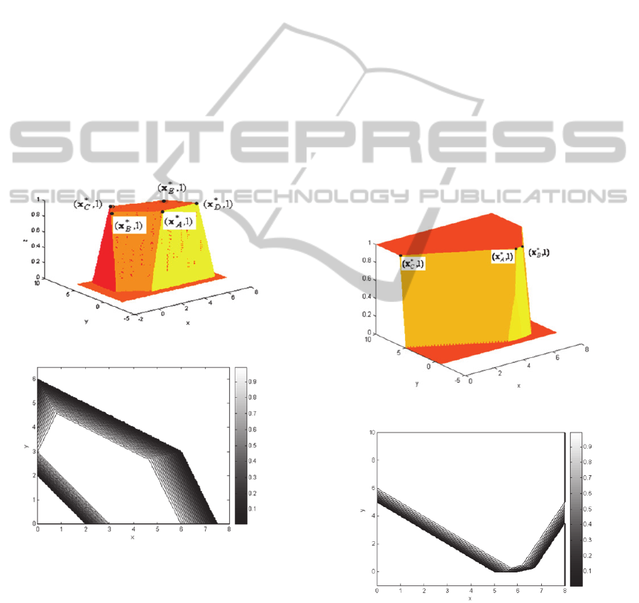
and 4-2 as
D
~
and its contour plot, respectively. The
set of optimal solutions,
)
~
(DNSC
, is the innermost
(white) 5-gone in Figure 4-2. In this figure the
alternative basic optimal solutions are the extreme
points:
*
A
x
,
*
B
x
,
*
C
x
,
*
D
x
and
*
E
x
. Also
)
~
(DNSC
=
, therefore
∗
1.
The line segment between
*
A
x
and
*
B
x
is the
objective function with the value 3, i.e.,
3
21
xx
. Clearly
21
xxz
attains the maximum value
in
*
E
x
.
Since the purpose of ZM is to obtain the best
value for
λ
, it does not prefer one of the AOS to
the others. Therefore, unless we check the value of
for all AOS, it is possible to introduce (for example)
*
A
x
to the DM as the optimal solution, ignoring the
fact that the best value for occurs at
*
E
x
.
Figure 4.1: The decision space of Example 4.1.
Figure 4.2: The contour plot of Figure 4-1.
When we solve this problem by WinQSB, a
cycling happens between
*
A
x
and
*
B
x
, hence only
these two solutions is shown, as the alternative basic
optimal solutions. Thus, the other three alternative
basic optimal solutions, those give better values for
, have been lost.
In the final example, ZM obtains an optimal
solution with a finite value for , whereas the
optimal value of is unbounded.
Example 4.2. Consider the following problem:
12
12
12
12
max
.. 2 5 10
~
5230
~
,0
zx x
st x x
xx
xx
Let
3,2,1,6
2100
pppb
. The geometric
approach gives Figures 4-3 and 4-4 as
D
~
and its
contour plot, respectively. The set of optimal
solutions,
)
~
(DNSC
, is the above region in figure 4-
3. Clearly the objective function
21
xxz
can
be increased in the white region to infinity. ZM does
not distinguish this case and presents a solution with
finite value. That is because the alternative optimal
basic solutions, are
)2857.0,7143.5(
*
A
x
,
)4762.0,1905.6(
*
B
x
and
)0.6,0(
*
C
x
, which
none of them gives the best value for .
Figure 4.3: The decision space of Example 4.2.
Figure 4.4: The contour plot of Figure 4-3.
5 THE IZM ALGORITHM
Safi et al., (2007) proposed the following algorithm
for improving ZM and called it "Improved
IllustratingtheDifficultiesofZimmermannMethodforSolvingtheFuzzyLinearProgrammingbytheGeometricApproach
437

Zimmermann Method" (IZM):
Step 1. for solving (2.1), take values
mipb
i
,...,1,0;and
0
, from the DM.
Step 2. Solve (2.5) for obtaining the optimal (x
*
,
*
).
Step 3. If problem (2.5) does not have any feasible
solution; Stop. If it has AOS, then go to step 4. Else,
z
*
= cx
*
is the best value for z. Stop.
Step 4. Solve the following LP problem:
*
*
max
.. (1 )
() (1 ) 1
0.
ii i
z
st b p
bpi ,,m
cx
cx
Ax
x
(5.1)
If problem (4.2) is unbounded, stop. Let x
**
be the
optimal solution of (4.2). If the set of all AOS is not
singleton go to Step 5. Else, Stop.
Step 5. (Efficiency, Guu and Wu, 1999) Solve:
0
**
**
max
. . ( ) ( ) 0,1,2,...,
0.
m
i
i
ii
i
s
tA A i m
xx
cx cx
x
REFERENCES
Bellman, R. E. and Zadeh L. A., 1970.Decision Making in
a Fuzzy Environment, Management Science 17, 141-
164.
Chanas, S., 1983. The use of Parametric Programming in
Fuzzy Linear Programming, Fuzzy Sets and Systems,
11, 243-251.
Guu, S. M. and Wu, Y. K., 1999. Two Phase Approach for
Solving the Fuzzy Linear Programming Problems,
Fuzzy Sets and Systems, 107, 191-195.
Rosenfeld, A., 1994. Fuzzy plane geometry:
triangles,Pattern Recognition Letters, 15, 1261-1264.
Safi M. R., Maleki, H. R. and Zaeimazad, E., 2007.A Note
on Zimmermann Method for Solving Fuzzy Linear
Programming Problem,Iranian Journal of Fuzzy
Systems, vol. 4, no. 2, 31-45
Safi M. R., Maleki, H. R. and Zaeimazad, E., 2007.A
Geometric Approach for Solving Fuzzy Linear
Programming Problems,Fuzzy Optimization and
Decision Making, 6, 315-336.
Tanaka H., Okuda, T.and Asai, K., 1974. On fuzzy
mathematical Programming, Journal of cybernetics
3(4), 37-46.
Verdegay, J. L., 1982. Fuzzy Mathematical Programming,
in: M.M. Gupta and E. Sanchez, Eds., Fuzzy
Information and Decision Processes, North-Holland,
Amsterdam, 231-236.
Zimmermann, H. J., 1976. Description and Optimization
of Fuzzy Systems,International Journal of General
Systems, 2, 209- 215.
IJCCI2012-InternationalJointConferenceonComputationalIntelligence
438
