
Data Dimensioning for Delay Differentiation Services in Regular
Plans for Mobile Clients
John Tsiligaridis
Heritage University, Math and Computer Science, 3240 Fort Road, Toppenish, WA, 98948, U.S.A.
Keywords: Broadcasting, Broadcast Plan, Mobile Computing.
Abstract: The broadcast problem including the plan design is considered. The data are inserted and numbered into
customized size relations at a predefined order. The server ability to create a full, regular Broadcast Plan
(RBP) with single and multiple channels after some data transformations is examined. The Basic Regular
Algorithm (BRA) prepares an RBP and enables users to catch their items while avoiding wasting energy by
their devices. In the case of multiple channels a dynamic grouping solution is proposed, called the Partition
Value Algorithm with Less Dimension (PVALD), under a multiplicity constraint. In order to provide an
RBP under relative delays a Dimensioning Algorithm (DA) is developed. The DA, with the criterion of
ratio, offers the differentiation of service. This last property, in addition to the self-monitoring, and self-
organizing, can be offered by servers today providing also channel availability and lower energy
consumption by using a smaller, number of channels, of equal bandwidth. Simulation results are provided.
1 INTRODUCTION
An efficient broadcast schedule program minimizes
the client expected delay, which is the average time
spent by a client before receiving the requested
items. The expected delay is increased by the size of
the set of data to be transmitted by the server. A lot
of work have been done for the data dissemination
with flat and skewed design (Acharya et al., 1995,
Yee et al., 2002, Ardizzoni et al., 2005, Bertossi et
al., 2004). For the flat design when the cycle
becomes large the users have to wait for long until
they catch the data in case they had lost them
previously. For the skewed design, the most
frequently requested data items should be put in fast
channels whereas the cold data can be pushed to
slow channels. Various methods have been
developed to partition the data according to their
popularity using dynamic programming (Yee et al.,
2002), and the heuristic algorithm VFk (Peng et al.,
2000). The minimum time broadcast problem has
been addressed by computing the minimum degree
spanning tree of directed acyclic graphs in (Yao et
al., 2008). The Min-Power broadcast problem in
wireless ad hoc networks has been answered by
assigning transmission range to each node (Hashemi
et al., 2007).
When the broadcast cycle has long size, the flat
scheduling needs many channels to avoid the user
delay. The regular design with the equal spacing
property (Acharya et al., 1995) can provide
broadcasting for single and multiple channels with
average waiting time less than the one of the flat
design. It also offers channel availability, and less
energy consumption while there is no need for use of
channels with different speeds.
For the regular design, the system works with a
number of channels that could be of the same speed.
The users of all sets, except for the last one, can get
their data from the same channel. Only the users of
the last set (the most unpopular set) have to switch
to another channel. The data are considered
homogenous or heterogeneous with multiples of a
basic size. Data can be sent by a single channel or a
set of channels. In this work the dynamic grouping
solution is developed by examining the possibility of
filling up an area starting from less values
especially from the cold set (the less dimension
principle, LDP).
In this paper, we study the problem of finding
the number of channels that can send a group of
data, while ensuring equal spacing of repeated
instances of items. The PVALD algorithm provides
a dynamic solution using the less dimension
principle with constraints. The constraints can be
applied with the use of certain criteria. The DA can
69
Tsiligaridis J..
Data Dimensioning for Delay Differentiation Services in Regular Plans for Mobile Clients.
DOI: 10.5220/0004119500690074
In Proceedings of the International Conference on Data Communication Networking, e-Business and Optical Communication Systems (DCNET-2012),
pages 69-74
ISBN: 978-989-8565-23-5
Copyright
c
2012 SCITEPRESS (Science and Technology Publications, Lda.)

discriminate the services according to relative delays
and provide the appropriate RBP. Both PVAMD and
DA provide servers with new approaches for service
discrimination. The paper is organized as follows. In
Section 2, the model description is given. In
Sections 3, 4, and 5 the BRA, the PVALD, and DA
are developed, respectively. Finally, simulation
results are provided in Section 6.
2 MODEL DESCRIPTION
2.1 The Relations in the Broadcasting
Plan
In our approach we consider three sets S
i
(i=1,2,3)
with their sizes S
is
so that S
3s
S
2s
S
1s
.The
possibility of providing full BP (it does not include
any empty slot) is examined iteratively using
relations starting from the last level of hierarchy S
3
.
The number of S
i
items (or items of multiplicity
(it_mu
i
)) will be sent at least one from S
3
,while for
the other two sets at least two. Given the size S
3s
,
S
2s
, S
1s
from the integer divisions of S
3s
, using
array (arr), we can create a set of relations S
div
(j< S
3s
), with different number of relations (n_rel) and
subrelations in each set (i-subrelation, i=1,2,3). We
create a set of relations including their subrelations
by considering items of different size from each set.
In this work it is considered that each relation has
three or four subrelations.
The following definitions are essential:
Definition 1: The size (or horizontal dimension) of
a relation (s_rel) is the number of items that belong
to the relation and it is equal to the sum of the size of
the three subrelations (s_rel=
3
1
_
i
i
subs
). The
number (or vertical dimension) of relations (n_rel)
with s_rel define the area of the relations (area_rel).
Example 1: The relation A=(a, b, c, d, f) has the
following three subrelations starting from the end
one; the 3-subrelation (f) with s_sub
3
= 1, the 2-
subrelation (b,c,d) with s_sub
2
= 3, and the 1-
subrelation (a) with s_sub
1
=1. The s_rel=5. The
integrated relation dimension (id) can be described
as id [1,2] or simply [1,2].
Definition 2: The area of the i-subrelation
(area_i_sub) is defined from its size (s_sub
i
) and
the number of the relations (n_rel) that are selected.
It is given by (s_sub
i
) x (n_rel).
Example 2: From a relation with s_rel=5 and if
n_rel=5 then the area of this relation is 5x 5. Hence
there are 25 locations that have to be completed.
Example 3: If two relations are: (1,2,3,5,6,7),
(1,3,4,8,9,10) with s_sub
3
=3, s_sub
2
=2, then : 2-
subrelation
1
=(2,3) and 2-subrelation
2
=(3,4). The
last two subrelations ((2,3),(3,4)) comes from S
2
={2,3,4} having 3 as repeated item.
Definition 3: A BP is full if it provides at least 2
repetitions of items and it does not include empty
slots in the area_rel. A BP is regular if it is full and
provides equal spacing property[1].
Definition 4: The number of items that can be
repeated in a subrelation is called item multiplicity
(it_mu) or number of repetitions (n-rep).
Definition 5: A subrelation i (i-subrelation) that
belongs to set S
i
is strong if, in its area, it can
provide the same number of repetitions of all the
items of a set (without empty slots) for all the
relations. The strong i-subrelations create strong
relations.
Definition 6: Integrated relations (or integrated
grouping) is when after the grouping, each group
contains relations with all the data of S
2
and S
1
. This
happens when: ( (2_subrelation) = S
2
)
(
(1_subrelation) = S
1
). See example 7 for details.
Grouping length(gl): The gl is a divisor of S
ks
(1,..,k). It is the n_rel that can provide homogenous
grouping.
Partition value (pv): It is the common divisor of S
is
(i=1,.., k) and gl for a given size of s_sum
i
. Hence:
pv
i
| S
is
and pv
i
| gl. Each set must have its own pv.
Example 4: If S
3s
=40, gl=20, considering that
s_sum
3
=8 then pv
3
=5 (=40/8) . Hence pv
3
| S
3s
and
pv
3
|gl
The criterion of homogenous grouping(chg): when
pv
i
| gl.
The criterion of multiplicity constraint(cmc) or
differential multiplicity: This happens if: it_mu
i+1
<
it_mu
i
(i= 1,..,n-1).
The criterion of PV (cpv): when: pv
i
< pv
j
(for i<j).
The chg along with cpv can guarantee the cmc for
different multiplicity (Theorem 1) and because of
that the cmc is not necessary to be examined.
The pv criterion can guarantee differential
multiplicity service. For having an RBP the criterion
of chg along with pv have to be held.
The number of channels (nc): S
k
/ gl (where S
k
is the
last set)
It is considered that a|b (a divides b) only when b
mod a =0 (f.e. 14 mod 2=0). The relation with the
maximum value of n_rel provides the opportunity
of maximum multiplicity for all items of S
2
and S
1
and finally creates the minor cycle of a full BP. The
major cycle is obtained by placing the minor cycles
on line.
DCNET 2012 - International Conference on Data Communication Networking
70

2.2 Some Analytical Results
Two basic Lemmas provide the possibility of the
FBP and RBP construction. The first deals with a
particular case of the S
2s
and S
3s
while the second is
a general case for every value of S
2s
, S
3s
. Proofs and
details for the case of empty slots BP are not
included in this work due to limited space.
After making sure that there is a RBP the data
from the array (the minor cycles for each array line)
are transferred to queues for broadcasting. For
multiple channels, the data from integrated relations
are grouping and then are broadcasting.
Example 5: The relation A= (a, b, c, d, f) has the
following three subrelations (s_sub
i
) starting from
the end one; the 3-subrelation (f) with s_sub
3
= 1,
the 2-subrelation (b,c,d) with s_sub
2
= 3, and the 1-
subrelation (a) with s_sub
1
=1. The size of relation
(s_rel) =5.
Lemma 1 (particular case): The basic conditions in
order from a set of data to have a regular broadcast
plan are: k= S
2s
/ S
3s
(1) and m= it_mu
2
= S
2s
/ k (2)
(item multiplicity).
Proof: For (1) if k= S
2s
| S
3s
then the k offered
positions can be covered by items of S
2s
and we can
take a full BP. From (2) m represent the number of
times (it_mu) that an item of S
2
will be in the
relation.
Example 6: (full BP) Consider the case of: S
1
= {1},
S
2
={2,3}, S
3
= { 4,5,6,7,8,9, 10, 11}. Moreover k=
S
2s
| S
3s
= 4(8/2) , and m=2(4/2) the it_mu
2
=2=4/2 .
The relations for the full BP are: (1,2,4,5), (1,3,6,7),
(1,2,8,9)(1,3,8,9). Since (s_sub
3
/ s_sub
2
) >1 we have
r_p =4 (2*2).
Example 7: Let’s consider S1 = {1}, S2 ={2,3,4,5},
S3 = {6,7,8,9, 10, 11,12,13}. Again, k=2(8/4), m=
it_mu
2
=2(4/2). Hence the FBP is (1,2,3,6,7),
(1,4,5,8,9),(1,2,3,10,11) ,(1,4,5,12,13). The
subrelations (2,3) (4,5).
Lemma 2 (general case): Given that S
2s
and S
3s
(and S
2s
S
3s
) with k
1
, k
2
their common divisors as:
k
1
= n/S
2s
(3) and k
2
= n/S
3s
(4) (where n= common
divisors of S
2s
and S
3s
): (a) if k
2
< S
2s
and k
2
/S
2s
(5) then there is an RBP with it_mu
2
= k
2
/S
2s
(b) if
k
2
> S
2s
and S
2s
/k
2
(6) then there is an RBP with
it_mu
2
= S
2s
/k
2
The RBP will have for both cases k
2
relations.
Proof: From (3) we get that the number of S
2
items
in a line s_sub
2
= k
1
/ S
2s
. From (4) we have s_sub
3
= k
2
/ S
3s
. If (5) is valid then it means that the k
2
positions (offered by S
3
) can be covered by k
2
/S
2s
items (it_mu
2
). If (6) is valid then it means that the
k
2
positions (offered by S3) can be covered by S
2s
/
k
2
Example 8: S
1
= {1}, S
2
={2,..,13}, S
3
= { 15,..,32}
, S
2s
= 12, S
3s
= 18. If n =3, k
1
= 3/12 =4, k
2
=
3/18=6, and k
2
/S
2s
= 6/12 = 2. Hence we have 6
relations and the 2-subrelations are:
(….,2,3,4,5,…),(…,6,7,8,9…),(…,10,11,12,13,…),
(….,2,3,4,5,…),(…,6,7,8,9…),(…,10,11,12,13,…).
If n=2, k
1
= 2/12 =6, k
2
= 2/18=9, and from k
2
/S
2s
=we have 9 12.
The less dimension principle, LDP, coming from
the diminishing of the size of cold set s_sum
k-1
(for
k sets ), the provides an opportunity to minimize the
delay (especially for the hot data) by using smaller
number of data in s_sum. If an RBP is feasible for
the low dimension of values this area can be
copied many times and provide an RBP for all the
available channels.
Example 9: Let us consider S
1s
=10,
S
2s
=20,S
3s
=40,S
5s
=120. Taking: d
1
=
5,d
2
=5,d
3
=5,d
4
=1 with s_sum = 16 the AWT
1
=
32(=4+5+5+1 + 4+5+5+1 + 1). For d
1
=
5,d
2
=5,d
3
=8,d
4
=1 with s_sum = 19 the AWT
1
= 38.
Considering smaller size of s_sum for an RBP
the size of PV
i
is increasing. Finally : from LDP the
AWT (LDP) is less that any other size of s_sum
Theorem 1 : Let us consider the case of multiple
channel allocation with different multiplicity of
sets (such as: S
1
, S
2
, S
3
). Then, if pvi|d4, the validity
of multiplicity constraint (it_mu
i+1
<it_mu
i
(i=1,..,k-
1) can be achieved from the pv criterion ( pv
i
<pv
i+1
, i<k, k=#sets). Similarly the pv criterion can
guarantee the multiplicity constraint criterion.
Proof: Lets prove that if pv
i
< pv
i+1
(1) then it_mu
i
>
it_mu
i+1
. (2). From (1) =>1/ pv
i
> 1/ pv
i+1
=> d
4
/ pv
i
> d
4
/ pv
i+1
. If (d
4
/ pv
i
) I, => it_mu
i
> it_mu
i+1
.
Following the reverse order we can go from (2) to
(1). Therefore, it is not necessary to examine the
multiplicity criterion and the pv criterion can
provide the multiplicity.
Example 10: Let’s consider again the same four
sets S
1
,S
2
,S
3
,S
4
with S
1s
=10, S
2s
=20,S
3s
= 40, S
4s
=120. If gl =20 (20 is a divisor of 120) then S
1s
/ gl,
S
2s
/ gl, gl / S
3s.
The chg exists. The number of
channels is: nc=120/20= 6. Considering s_sum1 = 5,
s_sum2=5,s_sum3=8 then pv
1
= 10/5=2, pv
2
=
20/5=4, pv
3
=40/8=5. We have pv
1
<pv
2
<pv
3
(pv
criterion) and since pv
1
|20 ,pv
2
|20,pv
3
|20 (or d
4
| pv
i
) I ) then the chg is valid and and an RBP can be
constructed. From all this process it is evident that
there is no need to test the cmc .
Theorem 2: If pv
i
(i<k, k =#sets) are analogous to a
i
the AWT
i
are also analogous to the a
i
and pv1 /
AWT1 = pv
2
/AWT
2
=…= pv
k
/ AWT
k-1
.
Proof: Let us consider k=4. and (pv
1
/a
1
) = (pv
2
/a
2
)
= (pv
3
/a
3
) (1)
Data Dimensioning for Delay Differentiation Services in Regular Plans for Mobile Clients
71

Finding AWT1: AWT1= s_sum*pv1 (= s_sum1-
1+s_sum2 + s_sum3 + s_sum1 -1= s_sum*a1 =
s_sum * pv1). In analogous way : AWT2 =
s_sum*a2 = s_sum*pv2, AWT3= s_sum*a3 =
s_sum* pv3,.., AWTk-1 =s_sum*a
k-1
=s_sum*pvk-1.
Taking the ratio: For AWT
1
/ a
1
= AWT2/ a
2
=
AWT
3
/ a
3
= ….= AWT
k-1
/ a
k-1
(2)
Dividing the ratios (1),(2) : pv
1
/ AWT
1
= pv
2
/AWT
2
=…= pv
k
/ AWT
k-1
.
Lemma: The LDP can provide an RBP with more #
of channels.
Example 11: For S1s=10,S2s=20,S3s=40, S4s=120,
and d
1
=5,d
2
=5,d
3
=5 the pv
1
=2,pv
2
=4,pv
3
=8 and
n_ch= 120/8=5. For d
1
=2,d
2
=2,d
3
=2
pv
1
=5,pv
2
=10,pv
3
=20 and n_ch=120/6=20.
3 THE BASIC REGULAR
ALGORITHM (BRA)
The BRA is based on the conditions to find a RBP
and provide opportunities for multiplicity on the
items of Si (i<n) and it is for a single channel
allocation.
4 THE PARTITION VALUE
ALGORITHM WITH LESS
DIMENSION (PVALD)
The PVAMD addresses the cases of minimum size
of integrated relations of all sets. It works with
neither grouping nor BRA. For k sets, PVALD
starts with the lower value of d
4
and s_sum
i
(i < k)
and d
k
=1.As soon as a BRP is feasible, so that the
criterion of homogenous grouping , pv and multiple
constraint are valid, the maximum number of
desired channels can be computed. The grouping is
used in order to adapt the RBP to the available
number of channels.
Example 12: Let us consider: S
1s
=10, S
2s
=20,S
3s
=
40, S
4s
=120 ,thr_ch=4. Considering : (a) for s_sum
1
=2, s_sum
2
=2,s_sum
3
=2 , (or [2,2,2]), d
4
=20, the
pv
1
= 5(10/2), pv
2
= 10 (20/2), pv
3
= 20 (40/2). Also
pv
1
| d
4
(=8=20/5), pv
2
|d
4
(=2=20/10), pv
3
|d
4
(=1=20/20) and pv
1
pv
2
pv
3
. The pv and
multiplicity criterion is valid. n_ch= 120/20=4>
thr_ch. So [2,2,2] with d
4
=20 can not provide the
desired RBP. (b) for s_sum1 =2,
s_sum2=2,s_sum3=2 , (or [2,2,2]), d4=40(=2*20),
the pv1 = 5(10/2), pv2= 10 (20/2), pv3= 20 (40/2).
Also pv
1
| d
4
(=8=40/5), pv
2
|d
4
(=4=40/10), pv
3
|d
4
(=2=40/20) and pv
1
pv
2
pv
3
. The pv and
PVALD input: S1,S2,S3,S4, Sis (i 4), n_ch:
the # of channels, m_n_ch: the max #
channels,a_ch:#avail.chan.
thr_ch: # of desired channels for an RBP
output: the homogenous grouping for multiple
channels
find the divisors set D
4
of S
4
(d
4
D
4
, increasing
order)
find the divisors of the S
1
,S
2
,S
3
(in increasing
order)
//D
3
for S
3
, D
2
for S
2
, D
1
for S
1
//d
3
D
3
, d
2
D
2
, d
1
D
1
for each s_sum (s_sum
i
, s_sum
i
= d
i
(i<4)) (a)
for each divisor (d
4
) of set S
4
(b)
for all S
i
(i4)
{ //define the s_sum
i
= d
i
(i<4)
s_sum
i
= d
i
(i<4)
pv
i
=S
is
/ s_sum
i
if pv
i
| d
4
(c)
{the chg criterion is valid,
“there is multiplicity”}
else {go to (b) }
if (pv
i
< pv
i+1
)
{“the pv criterion
is valid “
the m_n_ch = D
4
/ d
4
;
if (a_ch m_n_ch)
{ creation of an RBP for m_n_ch
channels}
else { grouping for an RBP with
a_ch}
else { go to (b)}
if (n_ch <thr_ch)
{d
4
= 2 *d
4
, go to (c) }
if (there is not an RBP for all d
4
–b-)
{go to (a) , new s_sum}
BRA: //input: the S
1
, S
2
, S
3
, num_set (=2)
//output: define k the max. # of relations (n_rel)
that can support a full BP
//variables: k,m,n I, n=common divisors of S
2s
and S
3s
km I and km > 1
//particular case
if (k= S
2s
| S
3s
) and m= it_mu
2
= S
2s
| k
{there is a full BP for S
2s
, with k lines
each item of S
is
(i=1,2) will be repeated for
m times,
//general case
if k
1
= n/S
2s
and k
2
= n/S
3s
(for given: S
2s
, S
3s
, n)
and k
2
/S
2s
{ there is an RBP with it_mu
2
= k
2
/S
2s
}
DCNET 2012 - International Conference on Data Communication Networking
72
multiplicity criterion is valid. n_ch= 120/40=3<
thr_ch. So [2,2,2] with d
4
=40 can provide the desired
RBP.
5 THE DIMENSIONING
ALGORITHM (DA)
The DA is very useful for finding the AWTi by
applying the Theorem 2. In addition any change to
the integrated relation (s_sum) or any subrelation
(s_subi) can easily be translated into delay. This is
very important for the server making decision
process and for having successful differentiation of
services.
Example13: Let’s consider: S1s=10,S2s=20,
S3s=40, S4s =120. The divisor of S4s are:
d4={10,20,30,40}. The purpose is to see for: AWT1/
2 = AWT2/4 = AWT3/8. For d
4
=10 and s_sum
1
=5,
s_sum
2
=5,s_sum
3
=5, the pv1 = 10/5 = 2,
it_mu1=10/2=5, pv2= 20/5 = 4, it_mu2= 10/4 I,
pv3=40/5=8 , and it_mu3= 10/8 I (pv criterion no
t valid). For d
4
=20 and s_sum
1
=5,
s_sum
2
=5,s_sum
3
=5, the pv1 = 10/5 = 2 ,
it_mu
1
=20/2=5, pv2= 20/5 = 4, it_mu
2
= 20/4 =5,
pv3=40/5=8 , and it_mu
3
= 40/8=5 (pv criterion is
valid). Also pv
1
< pv
2
<pv
3
(2<4<8) so the pv
criterion is valid.
The pv ratio is: pv
1
/2 = pv
2
/4=pv
3
/8 give the
AWT
1
/2= AWT
2
/4 =AWT
3
/8.
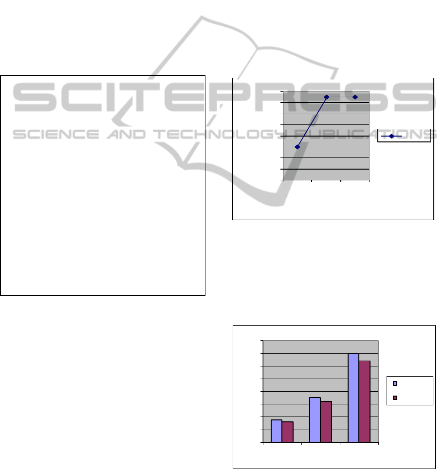
6 SIMULATION
For our simulation, Poisson arrivals are considered
for the mobile users’ requests. The items are
separated into four categories according to their
popularity using Zipf distribution. Two scenaria
have been developed:
Scenario 1: Considering S
4s
= 120,
S
3s
=60,S
2s
=40,S
1s
= 20. For the lower values of
s_sum (s_sum1=2, s_sum2=2,s_sum3=2 or [2,2,2]
(from integrated relation dimension –id-, using
PVAMD, we have the lower number of available
channels. For the other for two cases like: [5,5,5]
and [10,5,5] it is needed the same # of channels
since they have the same d
4
=8. It is considered that
s_sum
4
=1 for both cases.
0
2
4
6
8
10
12
14
16
id:[2,2,2]
id:[5,5,5]
id:[10,5,5]
# channels
#chan
Figure 1: The AWT for the PVAMD.
Scenario 2: Let us consider the same size of sets
as Scenario 1. The AWTi (i4) for [2,2,2] and
[5,5,5] have greater values for [2,2,2] since the
lower size of s_sumi can define greater values of pvi
and more times of repeated s-sum (including also the
s_sum
k
=1).
0
20
40
60
80
100
120
140
160
AWT1 AWT2 AWT3
id:{2,2,2]
id:[5,5,5]
Figure 2: The AWT for the different size of s_sum.
DA: input: s_sumi (i<k, k:#sets), PAi/ai : the
desired ratio
output: RBP with desired AWTi ratio
for each s_sum (s_sum
i
, s_sum
i
= d
i
(i<4)) (a)
for each divisor (d
4
) of set S
4
(b)
//find PVi
PAi = Sis / s_sumi
if pv
i
| d
4
{chg criterion is valid}
else {go to (b) }
if (pv
1
< pv
2
< …<pv
k-1
)
{the pv criterion is valid}
else {go to (b) }
if (pv
1
/a
1
= pv
2
/a
2
=…=pv
k-1
/a
k-1
)
{AWT
1
/a
1
= AWT
2
/a
2
=. . = AWT
k-1
/a
k-1
there is a RBP with the predefined ratio}
else {go to (b) }
if (there is not an RBP for all d
4
–b-)
{go to (a) , new s_sum}
Data Dimensioning for Delay Differentiation Services in Regular Plans for Mobile Clients
73

7 CONCLUSIONS
A new broadcast data model plan with a set of
algorithms has been presented. The PVAMD start
finding RBP by using the less dimension principle
with constraints. The DA provides opportunities for
finding the desired delays of a set of services. By
applying these algorithms the next generation
servers and their components with the scale up
possibilities, tools etc can enhance their self-
sufficiency, self-monitoring and they may address
quality of service, and other issues with minimal
human intervention.
REFERENCES
Acharya, S., Zdonik, F., Alonso, R., 1995. “Broadcast
disks: Data management for asymmetric
communications environments“, Proc. of the ACM
SIGMOD Int. Conf. on Management of Data, San
Jose, May 1995, 199-210
Yee, W., Navathe, S., Omiecinski, E., Jemaine, C., 2002. ”
Efficient Data llocation over Multiple Channels of
Broadcast Servers”, IEEE Trans. on Computers, vol.
51, No.10,Oct 2002.
Ardizzoni, E., Bertossi. A., Pinotti, M., Ramaprasad, S.,
Rizzi, R., Shashanka, M., 2005. ” Optimal Skewed
Data Allocation on Multiple Channels with Flat per
Channel”, IEEE Trans. on Computers , Vol. 54, No.
5, May 2005
Bertossi. A., Pinotti, M., Ramaprasad, S., Rizzi, R.,
Shashanka, M., 2004. “Optimal multi-channel data
allocation with flat broadcast per channel”,
Proceedings of IPDS’04, 2004, 18-27
Peng, W., Chen. M., 2000. ” Dynamic Generation of data
Broadcasting Programs for a Broadcast disk Array in a
Mobile Computing Environment”, Proc. of the 9
th
ACM International Conference on Information and
Knowledge Management (CIKM 2000), pp. 38-45
Yao, G., Zhu, D., Li, H., Ma. S., 2008. “ A polynomial
algorithm to compute the minimum degree spanning
trees of directed acyclic graphs with applications to the
broadcast problem”, Discrete Mathematics, 308(17),
3951-3959.
Hashemi, S., Rezapour, M., Moradi, A.,2007. ”Two new
algorithms for the Min-Power Broadcast problem in
static ad hoc networks” , Applied Mathematics and
Computation, 190(2) 1657-1668, 2007
DCNET 2012 - International Conference on Data Communication Networking
74
