Flexibility in Organic Systems

Remarks on Mechanisms for Adapting System Goals at Runtime

Christian Becker

, J

org H

ahner

and Sven Tomforde

System and Computer Architecture Group, Leibniz University Hannover, Appelstr. 4, 30167 Hannover, Germany

Lehrstuhl f

ur Organic Computing, Augsburg University, Eichleitnerstr. 30, 86159 Augsburg, Germany

Keywords:

Organic Computing, Flexibility, Machine Learning, Goal Exchange, Network Protocol Conﬁguration.

Abstract:

Within the last decade, technical systems that are capable of self-adaptation at runtime emerged as challenging

approach to cope with the increasing complexity and interconnectedness in today’s development and manage-

ment processes. One major aspect of these systems is their ability to learn appropriate responses for all kinds

of possibly occurring situations. Learning requires a goal function given by the user – which is subject to

modiﬁcations at runtime. In order to allow for ﬂexible manipulations of goals within the system’s operation

period, the learning component must be able to keep knowledge in order to respond to varying goals quickly.

This paper describes attempts to implementing ﬂexible learning in rule-based systems. First results show that

efﬁcient approaches are possible even in real-world applications.

1 INTRODUCTION

In recent years, technical systems capable of adapt-

ing themselves to changing environmental condi-

tions have gained increasing attention in industry and

academia. Driven by the insight that current design

approaches and the corresponding systems reach their

limits, a new paradigm for design processes has been

proposed. The main concept of this paradigm pos-

tulates to move parts of the control authority (e.g.

for conﬁguration aspects or the decision about most-

promising responses) from design time to runtime.

Hence, systems themselves become responsible for

ﬁnding appropriate reactions for occurring situations,

although these situations have not been anticipated by

an engineer in the ﬁrst place, cf. initiatives like Au-

tonomic (AC, (Kephart and Chess, 2003)) or Organic

Computing (OC, (Schmeck, 2005b)). Typically, this

increasing degree of autonomy is achieved by intro-

ducing self-* properties (Schmeck, 2005a) and by en-

abling automated learning capabilities – which results

in an increased adaptivity and a higher robustness of

the system compared to standard solutions.

In previous work (Tomforde, 2012), we intro-

duced a basic system design and framework to

achieve these desired organic capabilities. The ap-

proach is based on using population-based machine

learning techniques that limit the trial-and-error parts

of automated learning and thereby match safety-

restrictions of real-world systems. Usually, machine

learning systems are conﬁgured at design time by pro-

viding a certain goal (e.g. by applying a mathematical

function) which is to be approximated over time. Up-

coming OC systems face the demand of providing a

possibility to modify such goals at runtime as reac-

tion to changing user needs. We refer to this concept

as ﬂexibility, cf. (Schmeck et al., 2010).

Rule-based learning typically keeps track of a per-

formance estimation for each rule – the ﬁtness. This

ﬁtness is calculated and updated in response to ob-

served system behaviour and depends on the given

goal. After deﬁning the term ﬂexibility (section 2),

this paper discusses the need of novel mechanisms

for ﬂexibility in rule-based machine learning tech-

niques and introduces three different concepts (sec-

tion 3). Afterwards, these concepts are evaluated

within an exemplary application from the OC domain

(section 4). Section 5 summarised the paper and gives

an outlook to future work.

2 TERM DEFINITION:

FLEXIBILITY

Similar to various terms used in the context of self-

organised and organic systems, ﬂexibility has mani-

fold meanings in different research domains. Corre-

287

Becker C., Hähner J. and Tomforde S..

Flexibility in Organic Systems - Remarks on Mechanisms for Adapting System Goals at Runtime.

DOI: 10.5220/0004121002870292

In Proceedings of the 9th International Conference on Informatics in Control, Automation and Robotics (ICINCO-2012), pages 287-292

ISBN: 978-989-8565-21-1

 2012 SCITEPRESS (Science and Technology Publications, Lda.)

spondingly, it is measured according to the aspects

that are speciﬁc to the particular (application) domain.

For instance, various metrics are proposed to mea-

sure the ﬂexibility of manufacturing systems (Ben-

jaafar and Ramakrishnan, 1996; Hassanzadeh and

Maier-Speredelozzi, 2007; Shuiabi et al., 2005), pro-

gramming paradigms, architecture styles, and design

patterns (Eden and Mens, 2006) or different recon-

ﬁgurable hardware architectures (Compton, 2004).

There is no common deﬁnition, but the meaning of

the term as “adapting the system appropriately when

the goal is changed” is commonly agreed.

At a technical perspective and in the context of

OC, we typically rely on using Observer/Controller

patterns as basic system design (Schmeck, 2005b).

The most prominent variant is the Multi-level Ob-

server/Controller (MLOC) framework (Tomforde,

2012) which relies on using Learning Classiﬁer Sys-

tems (LCS) for online learning tasks. Even when ini-

tially testing LCS’ in artiﬁcial scenarios like the an-

imat exploring its environment (i.e. the Woods sce-

nario (Wilson, 1994)), the possibility of different

kinds of targets (here: artiﬁcial food) is already en-

visioned. In the context of this paper we will rely on

the OC terminology which was initially explained in

(Schmeck et al., 2010). Thereby, two concepts are

distinguished:

1. A system is characterised by its state z(t). If z(t)

changes due to a change of the system (e.g. bro-

ken components) or a change in the environmental

conditions (disturbance δ) and the system contin-

ues to show an acceptable behaviour, this system

is called a robust system.

2. In case of changes of the evaluation and accep-

tance criteria, the system’s state spaces that de-

ﬁne the targeted and accepted behaviour would be

modiﬁed. A system that is able to cope with such

changes in its behavioural speciﬁcation is called a

ﬂexible system.

The ﬁrst aspect is needed for most systems and

especially focused by diverse initiatives and research

domains like OC, AC, or Proactive Computing (Ten-

nenhouse, 2000). In contrast, the second aspect is

mostly left unregarded.

3 ORGANIC SYSTEMS AND

FLEXIBILITY

This section discusses the basic system design for

organic systems according to the Multi-level Ob-

server/Controller (MLOC) framework. Based on

this framework and the goal-related tasks within this

framework, we discuss technical issues and the corre-

sponding research problem for achieving ﬂexibility.

3.1 System Design

The MLOC framework for learning and self-

optimising systems as depicted in Figure 1 – ﬁrst in-

troduced in (Tomforde, 2012) – provides a uniﬁed

approach to automatically adapt technical systems

to changing environments, to learn the best adap-

tation strategy, and to explore new behaviours au-

tonomously. Figure 1 illustrates the encapsulation

of different tasks by separate layers. Layer 0 en-

capsulates the system’s productive logic (the System

under Observation and Control – SuOC). Layer 1

establishes a control loop with safety-based on-line

learning capabilities, while Layer 2 evolves the most-

promising reactions to previously unknown situa-

tions. In addition, Layer 3 provides interfaces to the

user and to neighbouring systems. Details on the

design approach, technical applications, and related

concepts can be found in (Tomforde, 2012).

Layer 3

Layer 0

Detector

data

Control

signals

User

System under Observation

and Control

Layer 1

Parameter selection

Observer

Controller

modified XCS

Layer 2

Offline learning

Observer

Controller

Simulator

Collaboration mechanisms

Monitoring Goal Mgmt.

Figure 1: System Design.

In the context of this paper, we conﬁne our regard

to those components that have to cover changes in the

user’s goals at runtime – in particular at Layer 1 and

Layer 2 of the architecture. At Layer 1 a modiﬁed

LCS serves as controller within the regulatory control

loop: it is responsible for adapting the SuOC’s pa-

rameter conﬁguration according to observed changes

in the environmental conditions. Due to safety-

restrictions in real-world systems, a standard LCS is

not applicable to the learning problem as it would op-

erate with too much freedom and relies strongly on

trial-and-error. Therefore, we modiﬁed the eXtended

Classiﬁer System (XCS) (Wilson, 1995) by remov-

ing the rule-generation parts and restricted the set of

possibly selectable rules. Details on these modiﬁca-

tions are given in (Tomforde, 2012) – they don’t in-

ﬂuence the powerfulness and operability of the XCS

algorithm. For understanding the technical impact of

ICINCO2012-9thInternationalConferenceonInformaticsinControl,AutomationandRobotics

288

allowing the user to change the overall system goal

at runtime, it is important to know that an XCS (and

so the modiﬁed variant) stores its knowledge and ex-

periences as rules in form of a basic 5-tuple. This

tuple contains the attributes condition (in which sit-

uation is the rule applicable?), action (what to do if

the rule is chosen?), prediction (what reward is ex-

pected if the rule is chosen?), error (how reliable is

the prediction?), and ﬁtness (what is the quality of the

rule?). Learning in an XCS is realised by modifying

the last three attributes using temporal difference al-

gorithms according to an observed reward – which de-

termines how well the user’s goals have been achieved

within the last evaluation cycle (typically referred to

as receiving a reward). If the user changes the goals

and thereby the reward function at runtime, the ex-

periences and knowledge stored within these evalua-

tion attributes don’t reﬂect the correct reward function

anymore. Hence, the XCS has to be further adapted in

order to allow for keeping its learning behaviour and

knowledge while simultaneously enabling an optimi-

sation process towards the new system goal. The dif-

ferent possibilities to deal with this problem are dis-

cussed in section 3.2.

While Layer 1 is responsible for learning online

from the observed system performance, Layer 2 re-

alises the OC concept of moving the trial-and-error

parts of learning to a sandbox. Similar to approaches

like Anytime Learning (Grefenstette and Ramsey,

1992), a simulation-coupled optimisation heuristic

evolves new rules in case of insufﬁcient knowledge at

Layer 1 and adds these novel rules to the rule-base of

the XCS. Again, this exploration of novel behaviour

in terms of rules needs a deﬁnition of good and bad

system performance – the user’s goals. First attempts

to deal with the related ﬂexibility problem are dis-

cussed in section 3.3.

3.2 Flexibility at Layer 1

Since Layer 1 of the architecture is concerned with

automatically improving the selection strategy over

time, its controller component is implemented us-

ing machine learning techniques – a modiﬁed XCS

in case of the MLOC framework. Each machine

learning technique uses a reward or ﬁtness function

f : K → [0, 1] to determine the strength of the used

parameter setting K ∈ K. Generalised versions with

f : K → B can also be found in literature. Since it

should be possible for the user to switch the system

goal at runtime, we need to extend the XCS to hold

a family of ﬁtness functions f

. The user is now ca-

pable of switching the system’s goal by changing α.

Starting from the simplest concept of “blowing up”

the existing concept, we investigated three different

approaches with increasing complexity to realise ﬂex-

ibility at Layer 1:

• Selective Approach. We extend the XCS to hold

multiple populations – one disjoint set for each

goal function. The XCS uses the population for

the currently set goal function and switches over

to another population when the user changes the

goal function of the OC system.

• Multi-dimensional Approach. Extend each clas-

siﬁer of the XCS to hold an array of 5-tuples –

one dimension for each goal function. The XCS

selects the 5-tuple according to the α of the cur-

rently set ﬁtness function. The difference to the

previous approach relies on which rules are stored

and the direct feedback for the evaluation criteria

even if another α is chosen.

• Cumulative Approach. Accumulate all goal

functions to a new one and use this new goal func-

tion to update the 5-tuple of the XCS.

We’ve chosen the following function f

Cumulative

for accumulating the different goal functions

Cumulative

(K) = E [ f

(K)]

−



max

{

(K)

}

− min

{

(K)

}



since a maximisation of this function results in a

minimisation of the difference between the maxi-

mum and the minimum while maximising the ﬁrst

moment. Consequently, all considered values are

in a small corridor around the ﬁrst moment.

3.3 Flexibility at Layer 2

In order to investigate ﬂexibility at Layer 2, we anal-

ysed three different approaches to modify the existing

optimisation heuristic to be ﬂexible in terms of OC:

• Multi-criterial Approach. Use a standard

Multi-criterial optimisation algorithm like the

S -Metric Selection Evolutionary Multi-Objective

Algorithm (SMS-EMOA) (Naujoks and Beume,

2005) and add the resulting set of rules to the pop-

ulation.

• Selective Approach. Minimise the amount of

evaluation calls and start optimisations for each

goal function with these minimised evaluation

calls.

• Cumulative Approach. Accumulate all goal

functions to a new one and optimise that new goal

function. We have chosen the same cumulative

function f

Cumulative

(K) as in Layer 1 (see 3.2).

FlexibilityinOrganicSystems-RemarksonMechanismsforAdaptingSystemGoalsatRuntime

289

Table 1: Variable parameters of the R-BCast protocol.

Parameter Standard conﬁguration

Delay 0.1 s

AllowedHelloLoss 3 messages

HelloInterval 2.0 s

δHelloInterval 0.5 s

Packet count 30 messages

Minimum difference 0.7 s

NACK timeout 0.2 s

NACK retries 3 retries

In contrast to the approach at Layer 1 of the archi-

tecture, the basic ﬂexibility concepts at Layer 2 can

be implemented using standard techniques in the ﬁrst

step. Therefore, the focus of this paper is conﬁned to

the Layer 1 aspects.

4 EVALUATION

The following section discusses the experimental in-

vestigation of the different ﬂexibility concepts for

Layer 1. The content is based on initial work as pub-

lished in (Becker, 2011).

4.1 Example Application

The basic design approach as presented in section 3.1

has been applied to various application scenarios,

including vehicular trafﬁc control, production, and

mainframe systems (Tomforde, 2012). In the con-

text of this paper, we turn our attention to the Organic

Network Control (ONC) (Tomforde et al., 2011) sys-

tem as example application. ONC has been developed

to dynamically adapt parameters of data communica-

tion protocols (i.e. buffer sizes, delays, or counters)

in response to changing environmental conditions. It

learns the best mapping between an observed descrip-

tion of the environment and the most promising re-

sponse in terms of a parameter conﬁguration.

Especially when applying ONC to broadcast al-

gorithms in mobile ad-hoc networks (MANET), we

demonstrated the signiﬁcant beneﬁt of the additional

ONC control. For instance, when applying ONC to

the R-BCast protocol (Kunz, 2003) ONC increased

the algorithm’s reliability and decreased the arising

overhead. Within this paper, we reuse the implemen-

tation of ONC controlling this R-BCast protocol to

demonstrate different ﬂexibility strategies. Table 1

lists the variable parameters of R-BCast and thereby

deﬁnes the conﬁguration space K. Details about the

parameters’ functionality and impact on the proto-

col’s logic as well as an explanation of the algorithm

can be found in (Kunz, 2003).

The online learning system relies on a situation

description as conditional part of each rule. In this

scenario, the distribution of other nodes in the direct

neighbourhood according to a sector-based model as

depicted in ﬁgure 2 serves as condition part, while the

parameter conﬁguration according to table 1 deﬁnes

the action part.

Figure 2: Environment representation.

4.2 Experimental Setup

We deﬁne the set of goal functions for the parameter

setting K ∈ K at the environment situation S by the

following family f

α,S

: K → [0, 1] with 0 < α < 1

α,S

(K) = α · f

PDR,S

(K) + (1 − α) · f

IOH,S

(K) (1)

where α is the weight for the sub goal functions

Packet-Delivery-Ratio (PDR) and Inverse-Overhead

(IOH). These goal functions comprise the most

prominent aspects when evaluating MANET-based

broadcast protocols – see e.g. (Williams and Camp,

2002) – and are deﬁned as follows:

• Packet-Delivery-Ratio f

PDR,S

(K):

AgentReceived

MaxSentMessages · #Nodes · #Senders

• Inverse-Overhead f

IOH,S

(K):

AgentSent

MacSent

We use the inverse function of the Overhead since our

optimisation problem should maximise its function.

This structure of the goal functions allows to change

them at runtime by simply manipulating the weight

factor α. An important reason for the selection of

those sub goal functions is the fact that a maximisa-

tion of the PDR is assumed to result in a minimisation

of the IOH and vice versa. We therefore have contrary

oriented goal functions which also increases the learn-

ing problem’s complexity as a simple coupling is not

possible with contrary aspects.

The evaluation of the three different approaches

uses the settings as depicted in table 2 for the simu-

lation. The ﬁrst eight hours rely on the goal function

ICINCO2012-9thInternationalConferenceonInformaticsinControl,AutomationandRobotics

290

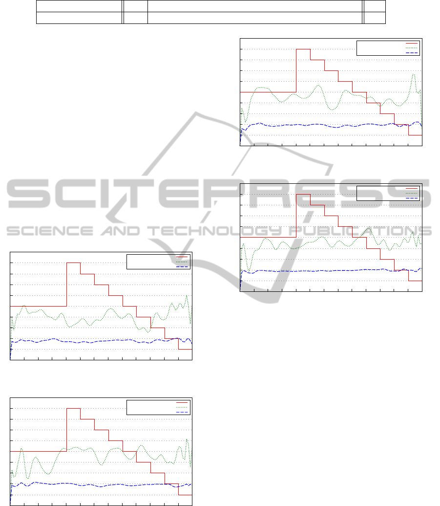
Table 2: Setting of the ONC simulation used for the evaluation.

Goal function by α 0.5 0.9 0.8 0.7 0.6 0.5 0.4 0.3 0.2 0.1 Σ

Duration in hours 8 2 2 2 2 2 2 2 2 2 26

0.5,S

to build up the XCS’ population and the corre-

sponding 5-tuples for each classiﬁer. After this build-

up time the XCS uses time slots of two hours for the

goal functions starting with f

0.9,S

and a decreasing α.

We used this setting to let the XCS ﬁnd a constant

population before changes in the goal function occur.

4.3 Results of the Evaluation

The ﬁgures 3 - 6 contain the evaluation results of the

simulation as explained in table 2 for the three differ-

ent approaches as presented in 3.2. They show the

Packet-Delivery-Ratio (green line) and the Inverse-

Overhead (blue line) in addition to the progress of

the weight factor α of the goal function f

α,S

(K) (red

line). Table 3 contains the averaged results. All ap-

proaches outperform the “ground-truth” of using the

protocol’s default values.

0.1

0.2

0.3

0.4

0.5

0.6

0.7

0.8

0.9

0 2 4 6 8 10 12 14 16 18 20 22 24 26

Alpha

Packet-Delivery-Ratio

Inverse-Overhead

Figure 3: Default values.

0.1

0.2

0.3

0.4

0.5

0.6

0.7

0.8

0.9

0 2 4 6 8 10 12 14 16 18 20 22 24 26

Alpha

Packet-Delivery-Ratio

Inverse-Overhead

Figure 4: Selective approach.

The cumulative approach performs worst com-

pared to the selective and the multi-dimensional ap-

proach. It was not possible to accumulate the contrary

character of the different goal functions to a mean-

ingful single value. Instead, the cumulative function

0.1

0.2

0.3

0.4

0.5

0.6

0.7

0.8

0.9

0 2 4 6 8 10 12 14 16 18 20 22 24 26

Alpha

Packet-Delivery-Ratio

Inverse-Overhead

Figure 5: Multi-dimensional approach.

0.1

0.2

0.3

0.4

0.5

0.6

0.7

0.8

0.9

0 2 4 6 8 10 12 14 16 18 20 22 24 26

Alpha

Packet-Delivery-Ratio

Inverse-Overhead

Figure 6: Cumulative approach.

Cumulative

results in a good rating of those classiﬁers

that a) perform better than the default values for all

goal functions but b) not optimal in any goal function.

The selective and multi-dimensional approaches

are similar in terms of the two goal functions. The

selective approach performs better for the Packet-

Delivery-Ratio while the multi-dimensional approach

results in a higher averaged value for the Inverse-

Overhead. In contrast, the averaged number of classi-

ﬁers needed to achieve this behaviour is different: the

multi-dimensional approach outperforms the selective

approach due to the disjunctive character of the latter

one’s population setup. In particular, the former ap-

proach does not rely on evolving a novel rule in each

occurring situation as it has broader knowledge from

other goal-aspects kept in the same population.

5 CONCLUSIONS

This paper discussed the need of novel mechanisms

to allow for ﬂexibility in organic systems. We named

different approaches from various domains where the

FlexibilityinOrganicSystems-RemarksonMechanismsforAdaptingSystemGoalsatRuntime

291

Table 3: Averaged rewards of the different approaches.

Approach Packet-Delivery-Ratio Inverse-Overhead

Default values 0.4006 0.1772

Selective 0.4509(+12.6%) 0.1923(+8.5%)

Multi-dimensional 0.4495(+12.2%) 0.1928(+8.8%)

Cumulative 0.4438(+10.8%) 0.1921(+8.4%)

term ﬂexibility is used and deﬁned what we want to

achieve in technical systems. Afterwards, we ex-

plained the need for novel techniques and mecha-

nisms to allow for a ﬂexible system behaviour in case

of learning and organic systems. Therefore, the basic

Observer/Controller pattern and its technical imple-

mentation have been mentioned.

The evaluation part introduced three different ap-

proaches to achieve ﬂexibility for the rule-based on-

line learning activities. According to the Organic

Network Control system as example application, we

compared the different concepts in a realistic envi-

ronment. Based on these ﬁrst insights, we will con-

tinue to ﬁnd solutions that keep the existing experi-

ence in case of changing goals and allow for an efﬁ-

cient learning. The paper showed that ﬂexibility is an

important issue and needs further research activities.

In upcoming OC systems, ﬂexibility will gain in-

creasing attention. Therefore, future work will explic-

itly have to cope with related mechanisms and strate-

gies. One possibility to investigate the problem sepa-

rated from the limitations and noisy effects of realistic

applications is the previously mentioned animat sce-

nario (see section 2). This scenario will serve as one

example and basis for more abstract investigations of

the ﬂexibility problem.

REFERENCES

Becker, C. (2011). Untersuchung von Mechanismen zur

technischen Umsetzbarkeit von Flexibilitaet in Organ-

ischen Systemen. Diploma thesis, Leibniz Universit

Hannover.

Benjaafar, S. and Ramakrishnan, R. (1996). Modeling,

Measurement and Evaluation of Sequencing Flexibil-

ity in Manufacturing Systems. Int. J. of Production

Research, 34:1195 – 1220.

Compton, K. (2004). Flexibility Measurement of Domain-

Speciﬁc Reconﬁgurable. In ACM/SIGDA Symp. on

Field-Programmable Gate Arrays, pages 155 – 161.

Eden, A. H. and Mens, T. (2006). Measuring software ﬂex-

ibility. IEE Proceedings - Software, 153(3):113–125.

Grefenstette, J. J. and Ramsey, C. L. (1992). An Approach

to Anytime Learning. In Proc. of the 9th Int. Workshop

on Machine Learning, pages 189–195.

Hassanzadeh, P. and Maier-Speredelozzi, V. (2007). Dy-

namic ﬂexibility metrics for capability and capacity.

Int. J. of Flexible Manufacturing Systems, 19:195 –

216.

Kephart, J. O. and Chess, D. M. (2003). The Vision of

Autonomic Computing. IEEE Computer, 36(1):41–

50.

Kunz, T. (2003). Reliable Multicasting in MANETs. PhD

thesis, Carleton University.

Naujoks, B. and Beume, N. (2005). Multi-objective optimi-

sation using S-metric selection: Application to three-

dimensional solution spaces. In Proc. of CEC’05,

pages 1282 – 1289. IEEE.

Schmeck, H. (2005a). Organic Computing. K

unstliche In-

telligenz, 3:68 – 69.

Schmeck, H. (2005b). Organic Computing – A new vision

for distributed embedded systems. In Proc. of the 8th

IEEE Int. Symp. on Object-Oriented Real-Time Dis-

tributed Computing, pages 201 – 203.

Schmeck, H., M

uller-Schloer, C., C¸ akar, E., Mnif, M., and

Richter, U. (2010). Adaptivity and self-organization

in organic computing systems. ACM Transactions on

Autonomous and Adaptive Systems (TAAS), 5(3):1–32.

Shuiabi, E., Thomson, V., and Bhuiyan, N. (2005). Entropy

as a measure of operational ﬂexibility. European Jour-

nal of Operational Research, 165(3):696 – 707.

Tennenhouse, D. (2000). Proactive computing. Communi-

cations of the ACM, 43(5):43–50.

Tomforde, S. (2012). Runtime adaptation of tech-

nical systems: An architectural framework for

self-conﬁguration and self-improvement at runtime.

udwestdeutscher Verlag f

ur Hochschulschriften.

ISBN: 978-3838131337.

Tomforde, S., Hurling, B., and H

ahner, J. (2011). Dis-

tributed Network Protocol Parameter Adaptation in

Mobile Ad-Hoc Networks. In Informatics in Control,

Automation and Robotics, volume 89 of LNEE, pages

91 – 104. Springer.

Williams, B. and Camp, T. (2002). Comparison of broad-

casting techniques for mobile ad hoc networks. In

Proc. of the 3rd ACM int. symp. on Mobile ad hoc net-

working & computing, pages 194–205. ACM.

Wilson, S. W. (1994). ZCS: A zeroth level classiﬁer system.

Evolutionary Computation, 2(1):1–18.

Wilson, S. W. (1995). Classiﬁer ﬁtness based on accuracy.

Evolutionary Computation, 3(2):149–175.

ICINCO2012-9thInternationalConferenceonInformaticsinControl,AutomationandRobotics

292