
Strictness of Rate-latency Service Curves
Ulrich Klehmet and Kai-Steffen Hielscher
Computer Networks and Communication Systems, University Erlangen, Martensstr. 3, 91058 Erlangen, Germany
Keywords:
Network Calculus, Blind Multiplexing, Strict Service Curve, Non-strict Service Curve.
Abstract:
Network Calculus (NC) offers powerful methods for performance evaluation of queueing systems, especially
for the worst-case analysis of communication networks. It is often used to obtain QoS guarantees in packet
switched communication systems. One issue of nowadays’ research is the applicability of NC for multiplexed
flows, in particular, if the FIFO property cannot be assumed when merging the individual flows. If a node
serves the different flows using another schedule than FIFO, the terms ’strict’ or ’non-strict’ service curves
play an important role. In this paper, we are dealing with the problems of strict and non-strict service curves
in connection with aggregate scheduling. In the literature, the strictness of the service curve of the aggregated
flow is reported as a fundamental precondition to get a service curve for the single individual flows at demul-
tiplexing, if the service node process the input flows in Non-FIFO manner. The important strictness-property
is assumed to be a unique feature of the service curve alone. But we will show here that this assumption is
not true in general. Only the connection with the concrete input allows to classify a service as curve strict or
non-strict.
1 INTRODUCTION
For systems with hard real time requirements, timeli-
ness plays an important role. This quality of service
(QoS) requirement can be found in all kinds of em-
bedded systems that permanently exchange data with
their environment, like automotive applications, real
time networks etc.
A mathematic-analytical performance evaluation
of such systems cannot be based on stochastic model-
ing like traditional queueing theory: the knowledge of
mean values is not enough. Worst-case performance
parameters like maximum delay of service times are
needed. In other words, one needs a mathematical
tool that guarantees performance figures in form of
bounding values which are valid in any case. Such a
tool is Network Calculus (NC), as a novel system the-
ory for deterministic queueing systems (Cruz, 1991),
(Le Boudec and Thiran, 2001).
The most important modeling elements of NC are
the arrival curve and service curve together with the
min-plus convolution. – We only present some fun-
damental definitions, more details can be found in
(Le Boudec and Thiran, 2001).
Let F be a flow of data (bits, messages, packets,
etc.) into a system S, let x(t) be the amount of data of
F arriving in time interval [0,t] and y(t) the amount
of data leaving S in time [0,t]. F is constrained by
an upper envelope and has the arrival curve α iff
x(t) − x(s) ≤ α(t − s) for all 0 ≤ s ≤ t, where α is
a non-negative, non-decreasing function.
A service curve β describes a lower bound for the out-
put y(t) and is offered by S iff β is a non-negative,
non-decreasing function with β(0) = 0 and y(t) ≥
(x⊗ g)(t) := inf
0≤s≤t
{x(s) + β(t − s)}.
⊗ is the convolution operator. The constraints given
by the arrival and service curves for a flow suffice to
calculate upper bounds on delay, backlog and output
of service nodes.
A commonly used arrival curve is the token bucket
constraint α
r,b
(t) = b + rt for t > 0 and zero other-
wise. α
r,b
provides an upper limit for traffic flows x(t)
with average rate r and instantaneous burst b.
A very important service curve is the rate-latency
function β(t) = β
R,T
(t) = R·[t−T]
+
:= R·max{0;t −
T}. The rate-latency function reflects a service ele-
ment which offers a minimum service of rate R af-
ter a worst-case latency of T. Worst-case perfor-
mance evaluation allows to abstract from the schedul-
ing strategies of complex systems.
In figure 1, the blue graph shows a token bucket ar-
rival curve α
r,b
and the green one reflects a rate-
latency service curve β
R,T
(t).
If the node or system serves the incoming data of
a flow in FIFO order, the following bound is com-
putable:
75
Klehmet U. and Hielscher K..
Strictness of Rate-latency Service Curves.
DOI: 10.5220/0004123800750078
In Proceedings of the International Conference on Data Communication Networking, e-Business and Optical Communication Systems (DCNET-2012),
pages 75-78
ISBN: 978-989-8565-23-5
Copyright
c
2012 SCITEPRESS (Science and Technology Publications, Lda.)
Theorem 1 (Delay Bound). Assume a flow con-
strained by arrival curve α(t) is passing a system with
service curve β(t). The maximum virtual delay d is
given as the supremum of all possible virtual delays
of data, i.e. it is defined as the supremum of the hor-
izontal deviation between arrival curve and service
curve:
d ≤ sup
s≥0
{inf{τ : α(s) ≤ β(s+ τ)}}.
The output flow is constrained by the arrival curve
α
∗
(t) = α ⊘ β := sup
s≥0
{α(t + s) − β(s)}
Figure 1 depicts this delay bound d and α
∗
.
Figure 1: Example for the bounds.
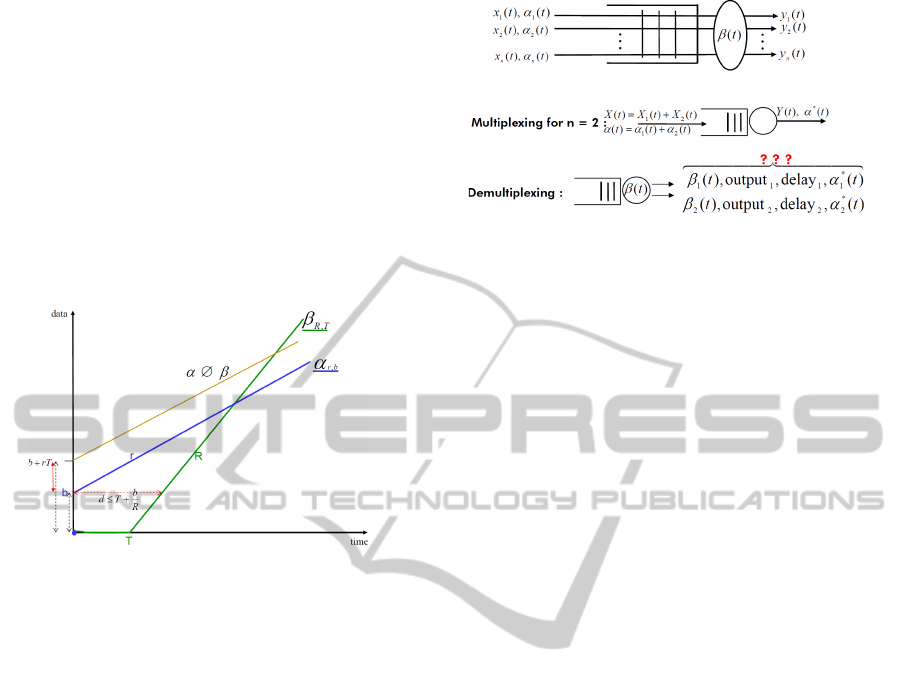
2 AGGREGATE SCHEDULING
Until now, we have only considered the service of a
single flow. But in real systems, aggregate scheduling
arises in many cases (Ying et al., 2008). In (Charny
and Le Boudec, 2000), delay bounds for general FIFO
networks are given.
When not only one single flow but many input
flows enter some kind of data processing system and
are then handled as a whole stream of data, we speak
of aggregate scheduling.
The main goal is to derive end-to-end bounds
(Schmitt et al., 2007). Important examples are Differ-
entiated Service domains (DS) of the Internet. In or-
der to address such class-based networks, we have to
consider multiplexing and aggregate scheduling. As-
sume that n flows enter a system or system node and
are scheduled by aggregation. According to (Fidler
and Sander, 2004), the aggregate input flow and ar-
rival curve are defined by addition of the input func-
tions respective arrival curves. When n = 2, the ag-
gregated input flow is x(t) = x
1
(t) + x
2
(t) and
α(t) = α
1
(t) + α
2
(t).
Figure 2 illustrates some important questions: Is
it possible to apply the same analysis, e.g. to calcu-
late the maximum delay using theorem 1 to the single
flows x
i
? Does there exists a service curve β
i
for the
Figure 2: Multiplexing of flows: input x
i
, output y
i
, arrival
& service curve α
i
, β = βaggr.
individual flow x
i
that allows us to use theorem 1 to
find the maximum delay for the single flows x
i
, when
we assume that the aggregate flowis serviced and sub-
sequently demultiplexed?
The answers to these questions depend on the type
of multiplexing, i.e. in which manner the aggregate
scheduling is done: FIFO (as e.g. in (Rizzo, 2008)),
priority-scheduling, multiplexing by unknown arbi-
tration between the flows etc. Together with the par-
ticular scheduling strategy, one has to take the ser-
vice curve of the aggregate flow into consideration.
For instance in case of FIFO, the family of func-
tions β
1
θ
(t) := [β(t) − α
2
(t − θ)]
+
if t > θ (otherwise
β
1
θ
(t) := 0) is a service curve for the single flow x
1
:
y
1
≥ x
1
⊗ β
1
θ
, where y
1
is the output of flow x
1
(as-
sumed α
2
is arrival curve of flow x
2
, θ ≥ 0, β
1
θ
is non-
negative and non-decreasing).
However, if no knowledge about the choice of ser-
vice between the flows is present, then we speak of
arbitrary multiplexing (Schmitt et al., 2008) or blind
multiplexing, and the situation is more complex. Now,
the distinction between strict and non-strict aggregate
service curves playsan importantrole (Le Boudec and
Thiran, 2001).
Theorem 2 (Blind Multiplexing.). Consider a node
serving the flows x
1
and x
2
, with some unknown arbi-
tration between the two flows. Assume the node guar-
antees a strict service curve β to the aggregate of the
two flows and that flow x
2
is bounded by α
2
. Define
β
1
(t) := [β(t) − α
2
(t)]
+
. If β
1
is wide-sense increas-
ing, then it is a service curve for flow x
1
.
A service curve is called strict when the following
definition holds:
Definition 1 (Strict Service Curve). A system S offers
a strict service curve β to a flow if during any back-
logged period [s,t] of duration u = t − s the output y
of the flow is at least equal to β(u), i.e. y(t) − y(s) ≥
β(t − s), or equivalently y(z) ≥ β(z) ∀z ∈ [s, t].
Of course, any strict service curve is also a regular
service curve.
DCNET2012-InternationalConferenceonDataCommunicationNetworking
76
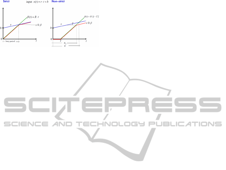
Figure 3: Strict and non-strict server.
Example 1. Figure 3 shows a token bucket-like in-
put x = rt + b and a service curve β(t) = R· t on the
left-hand side. Here, the output y(u) ≥ β(u) in all
backlogged periods u less than or equal to the busy
period. Thus, in this scenario, the service curve β is
strict.
If we change the service curve β(t) = R · t to the
rate-latency service curve β
R,T
(t) = R· [t − T]
+
at the
right-hand side of figure 3, we get a non-strict service
curve. The backlogged time starts at time zero, but
never ends, since all input data of x remains within
the system for time T before leaving with rate R. The
definition of the service curve specifies the output y
as y(t) ≥ (x⊗ β)(t). Indeed, it is valid that the output
y(u
0
) ≥ β
R,T
(u
0
), but this is not guaranteed regarding
the backlogged period u > u
0
. Thus, it is possible that
y(u) 6≥ β
R,T
(u) as (x⊗β
R,T
)(u)−(x⊗ β
R,T
)(0) = (x⊗
β
R,T
)(u) < β
R,T
(u) = β
R,T
(u) − β
R,T
(0) if T > 0. In
this scenario, the service curve β is non-strict.
Example 1 already provokes the question: Is there
a class of service functions that always have the prop-
erty of being strict or non-strict? In the literature,
the service curve β
R,T
(t) = R· [t − T]
+
(or even any
convex service curve) is often used as strict service
curve per se, for instance in (Bouillard et al., 2007).
But we will see that the strictness or non-strictness is
not based on the service curve or a class of service
curves alone, but it depends on both the service curve
β and the respective input flow x. That means that we
have to check whether the strictness is given for the
aggregated input flow before applying the important
theorem 2 in many aggregated flow-situations, i.e. we
need to proof the condition
y(t) ≥ β(t), ∀t ∈ backlogged period u.
Concerning this matter now, at least for most prac-
tical applications using token bucket like input flows
and rate-latency service curves β
R,T
, we will provide
here some characterizations.
Theorem 3 (Non-strict Functions.). Consider a sys-
tem with rate-latency service curve β
R,T
and token
bucket arrival curve α
r,b
, holding the conditions r < R
and T > 0. The service curve β
R,T
cannot be strict, if
the input flow x(t) is a strictly increasing function.
Proof: Assume β
R,T
is strict.
α
∗
(t) = α ⊘ β := sup
s≥0
{α(t + s) − β(s)}, here
α
∗
(t) = r(t+T)+b. Because r < R, there is a point in
time t
s
,such that β
R,T
(t
s
) = α
∗
(t
s
) and β
R,T
(t) > α
∗
(t)
if t > t
s
, i.e. ∀ t
0
> t
s
: β
R,T
(t
0
) − α
∗
(t
s
) ≥ α
∗
(t
0
) −
α
∗
(t
s
) ⇒ ∆β
R,T
= β
R,T
(t
0
) − β
R,T
(t
s
) ≥ α
∗
(t
0
) −
α
∗
(t
s
) = ∆α
∗
.
Since x is strictly increasing, and latency T > 0, it
holds for any t
0
> t
s
: u := t
0
− t
s
is a backlogged pe-
riod.
β
R,T
is supposed to be strict, so output y(u) ≥
β
R,T
(u) = β
R,T
(t
0
) − β
R,T
(t
s
) ≥ α
∗
(t
0
) − α
∗
(t
s
) =
α
∗
(t
0
− t
s
). But this is a contradiction to α
∗
being an
arrival curve for output y. Therefore, the assumption
is wrong, i.e. β
R,T
is non-strict. 2
Unfortunately, the feature of being a non-strictly
increasing input x is not a sufficient condition for a
strict service curveβ
R,T
: Using the same token bucket
arrival curve α
r,b
and rate-latency service curve β
R,T
,
one can find non-strictly increasing input functions x
that make the service curve β
R,T
both strict and non-
strict. The following examples will show this.
Example 2. Be α
r,b
:= 1, 5t + 5 for t > 0 and zero
else and β
R,T
:= 2(t − 2)
+
. Be the input x such that
it is first identical with α
r,b
and then stagnates at time
t
′
. Here, the parameter t
′
is computed using the equa-
tion α
r,b
(t) = β
R,T
(t + T). This guarantees that no
displacement of the β
R,T
-graph within the convolution
graph of x ⊗ β
R,T
occurs: 1, 5t + 5 = 2((t + 2) − 2).
t = t
′
= 10 fulfills this equation. So, we define the
input as
x :=
0 : t ≤ 0
1, 5t + 5 : t ≤ 10
20 : else
Result: The service curve β
R,T
is strict.
Next, only the input x is changed a little bit from
x to a ˜x, and the service curve β
R,T
= 2(t − 2)
+
is
automatically transformed to be non-strict:
Be ˜x :=
0 : t ≤ 0
0, 75t + 2, 5 : t ≤ 10
10 : else
(˜x is still monotonous and non-strictly increasing.)
Result: β
R,T
is non-strict now with this input ˜x.
Figure 4 demonstrates both situations.
Due to the previous demonstration, the following
characterization of input functions can be given:
All input functions x of the form (or multiple pat-
tern of this)
x :=
mt + n : t ≤ t
0
≤
´
t
const : else
StrictnessofRate-latencyServiceCurves
77
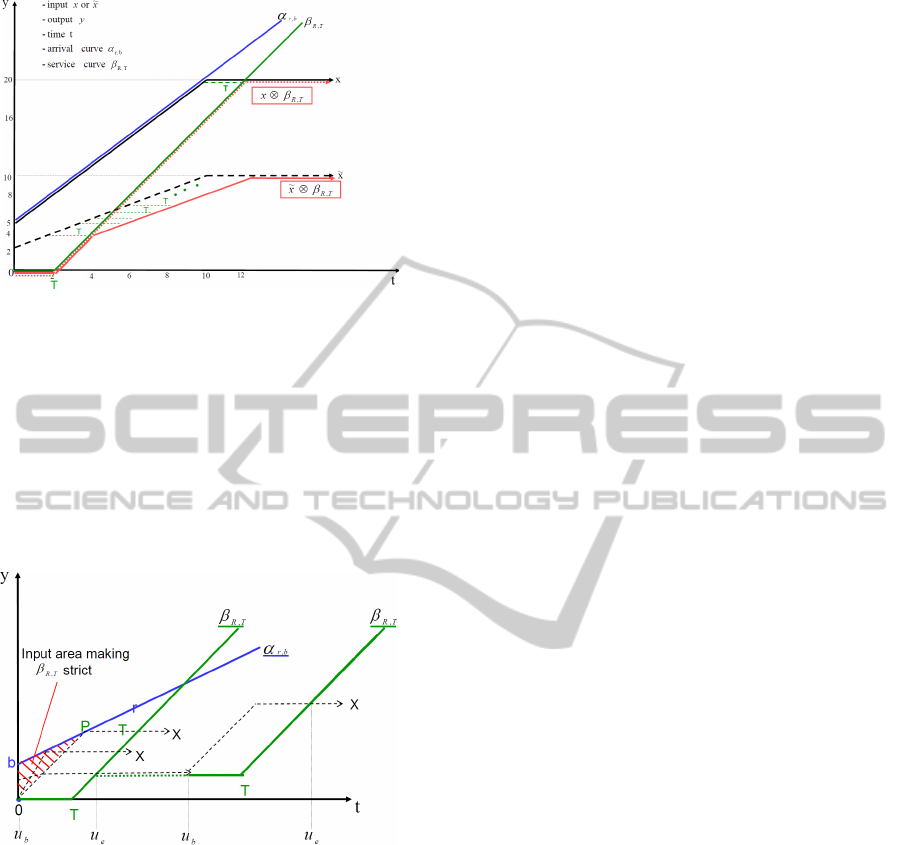
Figure 4: Input x changed to ˜x causes non-strictness.
cause the service curve β
R,T
to be strict, when the
constant part of x starts within the red-dashed trian-
gle with the corner points 0bP or on the edge of as
shown in figure 5.
Here, u
b
is the begin and u
e
the end of the back-
logged period, b is the burst size of the arrival curve
α
r,b
and P = P(
´
t, ´y) with
´
t: α
r,b
(
´
t) = β
R,T
(
´
t + T), i.e.
the intersection of α
r,b
with the parallel line to β
R,T
,
given by the curve y = Rt.
Figure 5: Input area making β
R,T
strict.
3 CONCLUSIONS
In this paper, we illustrated one particular problem
that arises in situations of blind multiplexing when
using the methods of network calculus: The construc-
tion of a service curve for the single output after de-
multiplexing an aggregated flow x = x
1
+ x
2
requires
the strictness of the aggregated service curve.
In publications like (Bouillard et al., 2007) or
(Schmitt et al., 2008) and others, it is assumed that
the rate latency service curve (often used as an aggre-
gated service curve) fulfills the strictness property.
However,we showed that the feature of being strict or
non-strict is not a unique feature of the service curve
alone. Only in combination with the concrete input or
at least with a special class of inputs, we can decide
whether a service curve is strict or non-strict.
REFERENCES
Bouillard, A., Gaujal, B., and Lagrange, S. (2007). Optimal
routing for end-to-end guarantees: the price of multi-
plexing. In Valuetools ’07, Nantes.
Charny, A. and Le Boudec, J.-Y. (2000). Delay Bounds in a
Network with Aggregate Scheduling. Springer Verlag
LNCS 1922.
Cruz, R. (1991). A calculus for network delay, part i: Net-
work elements in isolation. IEEE Trans. Inform. The-
ory, 37-1:114–131.
Fidler, M. and Sander, V. (2004). A parameter based ad-
mission control for differentiated services networks.
Computer Networks, 44:463–479.
Le Boudec, J.-Y. and Thiran, P. (2001). Network Calculus.
Springer Verlag LNCS 2050.
Rizzo, G. (2008). Stability and Bounds in Aggregate
Scheduling Networks. Ecole Polytechnique Federale
De Lausanne, PhD Thesis.
Schmitt, J., Zdarsky, F., and Fidler, M. (2007). Delay
Bounds under Arbitrary Multiplexing. Technical Re-
port, 360/07.
Schmitt, J., Zdarsky, F., and Martinovic, I. (2008). Improv-
ing Performance Bounds in Feed-Forward Networks
by Paying Multiplexing Only Once. In Measurements,
Modelling and Evaluation of Computer and Com-
munication Systems(14th GI/ITG Conference), Dort-
mund.
Ying, Y., Guillemin, F., Mazumdar, R., and Rosenberg, C.
(2008). Buffer overflow asymptotics for multiplexed
regulated traffic. Performance Evaluation, 65-8.
DCNET2012-InternationalConferenceonDataCommunicationNetworking
78
