Simulated Annealing based Parameter Optimization of Time-frequency
ε-filter Utilizing Correlation Coefficient
Tomomi Matsumoto
1
, Mitsuharu Matsumoto
2
and Shuji Hashimoto
1
1
Department of Applied Physics, Waseda University, 55N-4F-10A, 3-4-1 Okubo, Shinjuku-ku, Tokyo, Japan
2
The Education and Research Center for Frontier Science, University of Electro-communications, 1-5-1, Chofugaoka,
Chofu-shi, Tokyo, Japan
Keywords:
Simulated Annealing, Parameter Optimization, Noise Reduction, ε-filter, Nonlinear Filter, Time-frequency
ε-filter.
Abstract:
Time-Frequency ε-filter (TF ε-filter) can reduce different types of noise from a single-channel noisy signal
while preserving the signal that varies drastically such as a speech signal. It can reduce not only small station-
ary noise but also large nonstationary noise. However, it has some parameters whose values are set empirically.
So far, there are few studies to optimize the parameter of TF ε-filter automatically. In this paper, we employ
the correlation coefficient of the filter output and the difference between the filter input and output as the
evaluation function of the parameter optimization. We also propose an algorithm to set the optimal parameter
of TF ε-filter automatically. The experimental results show that we can obtain the adequate parameter in TF
ε-filter automatically by using the proposed method.
1 INTRODUCTION
Noise reduction plays an important role in speech
recognition and individual identification. When
we consider the instruments like hearing-aids and
phones, noise reduction for a single-channel signal
is required. The spectral subtraction (SS) is a well-
known approach for reducing the noise signal of the
monaural-sound (Boll, 1979; Lim, 1978). It can re-
duce the noise effectively with the simple procedure.
However, it can handle only the stationary noise.
It also needs to estimate the noise spectrum in ad-
vance. Although noise reduction utilizing Kalman
filter has also been reported (Kalman, 1960; Fuji-
moto and Ariki, 2002), the calculation cost is large.
Some authors have reported a model based approach
for noise reduction (Daniel et al., 2006). In this ap-
proach, we can extract the objective sound by con-
structing the sound model in advance. However, it is
not applicable to the signals with the unknown noise.
There are some approaches utilizing comb filter (Lim
et al., 1978). In this approach, we firstly estimate the
pitch of the speech signal, and reduce the noise signal
utilizing comb filter. However, the estimation error
results in the degradation of the speech quality espe-
cially in case of consonant.
Harashima et al. have reported a nonlinear filter
named ε-filter , which can reduce noise while preserv-
ing the signal (Harashima et al., 1982) . We label it
“TD ε-filter” as it handles signal shape in time do-
main. TD ε-filter is simple and has some desirable
features for noise reduction. It does not require the
model not only of the signal but also of the noise
in advance. It is easy to be designed and the calcu-
lation cost is small. It can reduce not only the sta-
tionary noise but also the nonstationary noise. How-
ever, it can reduce only the small amplitude noise
in principle. To solve the problems, the method la-
beled time-frequency ε-filter (TF ε-filter) was pro-
posed (Abe et al., 2007). TF ε-filter is an improved
ε-filter applied to the complex spectra along the time
axis in time-frequency domain. By utilizing TF ε-
filter, we can reduce not only small amplitude sta-
tionary noise but also large amplitude nonstationary
noise. However, TF ε-filter has some parameters and
we need to set them adequately based on empirical
control. Moreover, as we only have a single-channel
noisy signal, it is difficult to evaluate whether the pa-
rameter is optimal or not. We cannot know the differ-
ence between the original signal and the filter output
from the observed signal. So far, there are few studies
on the appropriateness of the parameter setting of TF
ε-filter.
Based on the above prospects, we proposed an ap-
237
Matsumoto T., Matsumoto M. and Hashimoto S..
Simulated Annealing based Parameter Optimization of Time-frequency e-filter Utilizing Correlation Coefficient.
DOI: 10.5220/0004126602370241
In Proceedings of the International Conference on Signal Processing and Multimedia Applications and Wireless Information Networks and Systems
(SIGMAP-2012), pages 237-241
ISBN: 978-989-8565-25-9
Copyright
c
 2012 SCITEPRESS (Science and Technology Publications, Lda.)

proach to set the parameter (Abe et al., 2009). In
this method, as a simple criterion, we assume that the
signal and noise are noncorrelated. And we employ
the correlation coefficient of the filter output and the
difference between the input signal and the filter out-
put to set the parameter adequately. In this study, we
confirmed that the correlation became almost mini-
mal when the error was minimal. However, as the
correlation has many local minimum, we could not
employ gradient method. To solve the problem, we
use simulated annealing to set the parameter in this
paper. When we utilize the proposed method, we can
set the parameter adequately without the information
about the noise and the signal. In Sec.2, we explain
TF ε-filter to clarify the problem. In Sec.3, we de-
scribe the algorithm of the method to determine the
parameter adequately. In Sec.4, we show the exper-
imental results. Experimental results show that the
proposed method can estimate the optimal parameter
of the TF ε-filter. Conclusions are given in Sec.5.
2 TIME-FREQUENCY ε-FILTER
In this section, we briefly describe the TF ε-filter algo-
rithm. TF ε-filter is an improved ε-filter applied to the
complex spectra along the time axis in time-frequency
domain.
Let us define x
k
as the input signal sampled at time
k. In TF ε-filter, we firstly transform the input sig-
nal x
k
to the complex spectra X
κ,ω
by short term
Fourier transformation (STFT). κ and ω represent the
time frame and the angular frequency in the time-
frequency domain, respectively. κ and ω are integer
numbers. Next we execute a TF ε-filter, which is an ε-
filter applying to complex spectra along the time axis
in the time-frequency domain. In this procedure, Y
κ,ω
is obtained as follows:
Y
κ,ω
=
Q
∑
i=−Q
1
2Q+ 1
X
0
κ+i,ω
, (1)
where
X
0
κ+i,ω
(2)
=

X
κ,ω
(||X
κ,ω
| − |X
κ+i,ω
|| > ε)
X
κ+i,ω
(||X
κ,ω
| − |X
κ+i,ω
|| ≤ ε),
and ε is a constant. We define the window size of ε-
filter as 2Q+ 1. Then, we transformY
κ,ω
to the output
signal y
k
by inverse STFT.
By utilizing TF ε-filter, we can reduce not only small
amplitude stationary noise but also large amplitude
nonstationary noise because the noise power is dis-
tributed in wide frequency range even when the noise
has large amplitude in time domain. It does not re-
quire either the model of the signal or that of the noise
in advance. It is easy to be designed and the calcula-
tion cost is small (Abe et al., 2007).
3 AUTOMATIC PARAMETER
OPTIMIZATION UTILIZING
CORRELATION COEFFICIENT
As described in the previous section, when the TF ε-
filter is employed, we need to set ε value adequately
to reduce the noise. However, we cannot estimate the
optimal parameter because the noise and signal are
not known throughout all the procedures.
To solve the problem, we pay attention to the cor-
relation of the target signal and the noise signal. We
make the following assumption concerning the target
signal and noise signal:
• Assumption 1. The target signal is noncorrelated
with the noise signal.
Let us define s
k
and n
k
as the objective signal and
the noise signal, respectively. Let R(s
k
,n
k
) be the cor-
relation coefficient of s
k
and n
k
described as follows:
R(s
k
,n
k
)
=
L
∑
k=1
(s
k
− s
k
)(n
k
− n
k
)
s
L
∑
k=1
(s
k
− s
k
)
2
s
L
∑
k=1
(n
k
− n
k
)
2
, (3)
where L is the data length. s
k
and n
k
represent the
averages of s
k
and n
k
, respectively. s
k
and n
k
are de-
scribed as follows:
s
k
=
1
L
L
∑
k=1
s
k
. (4)
n
k
=
1
L
L
∑
k=1
n
k
. (5)
When L is large enough, it is expected that the fol-
lowing equation is satisfied under assumption 1:
R(s
k
,n
k
) = 0. (6)
As described above, s
k
and n
k
are unknown
throughout the filtering procedures. Instead of s
k
and
n
k
, we consider the correlation coefficient of the fil-
ter output and the difference between the input signal
and the filter output. Let us consider x
k
and y
k
as the
input signal and the output signal of TF ε-filter, re-
spectively. x
k
can be described as follows:
x
k
= s
k
+ n
k
. (7)
SIGMAP2012-InternationalConferenceonSignalProcessingandMultimediaApplications
238

When the TF ε-filter can reduce the whole noise,
while it preserves the signal completely, the filter out-
put y
k
equals the signal s
k
. The noise n
k
can be de-
scribed as follows:
n
k
= x
k
− s
k
= x
k
− y
k
. (8)
Although actual TF ε-filter does not reduce the
whole noise and reduces the signal, if ε value is set
optimally, it is expected that the correlation of y
k
and
x
k
− y
k
becomes smaller than that of y
k
and x
k
− y
k
in other ε. Hence, the optimal parameter ε
opt
can be
obtained as
ε
opt
= argmin
ε
|R(y
k
,x
k
− y
k
)|, (9)
where
R(y
k
,x
k
− y
k
) (10)
=
L
∑
k=1
(y
k
− y
k
)(x
k
− y
k
− x
k
− y
k
)
s
L
∑
k=1
(y
k
− y
k
)
2
s
L
∑
k=1
(x
k
− y
k
− x
k
− y
k
)
2
,
where x
k
and x
k
− y
k
represent the average of x
k
and
x
k
− y
k
, respectively. x
k
and x
k
− y
k
are described as
follows:
x
k
=
1
L
L
∑
k=1
x
k
. (11)
x
k
− y
k
=
1
L
L
∑
k=1
(x
k
− y
k
). (12)
To obtain the adequate parameter automatically,
we utilize the simulated annealing. The process of
the simulated annealing is represented as follows:
Step1 We set ε at the initial parameter ε
0
and the
initial temperature T.
Step2 We calculate the initial solution y
k
(ε
0
).
Step3 We repeat the following process until the ter-
mination condition is fulfilled.
1. We randomly choose the ε
0
which satisfies: ε−
a < ε
0
< ε+ a. Where a is the constant number
which constrains ε
0
within the neighborhood of
ε.
2. We calculate the |R(y
k
(ε),x
k
− y
k
(ε))| and
|R(y
k
(ε
0
),x
k
− y
k
(ε
0
))|
3. If |R(y
k
(ε
0
),x
k
− y
k
(ε
0
))| ≤ |R(y
k
(ε),x
k
−
y
k
(ε))| , ε is replaced to ε
0
. Otherwise ε is
replaced to ε
0
with probability e
−(y
k
(ε
0
)−y
k
(ε))/T
.
Step4 Step 2 and 3 are repeated for a while. If ε value
is kept despite the procedure, the terminal condi-
tion of iteration is fulfilled. And we regard the ε
as the optimized solution. Otherwise we decrease
T and go back to the Step2.
As the initial parameter ε
0
, we use the value described
by the following equation.
ε
0
= σ(X
κ,ω
) (13)
where
σ(X
κ,ω
) =
1
M
M
∑
ω=1
s
1
N
N
∑
κ=1
(X
κ,ω
− X
κ,ω
)
2
, (14)
where M and N represent the number of frequency
resolution and the number of the time frame, respec-
tively. Eq. 14 represents the mean along the fre-
quency axis of the standard deviation along the time
axis of X
κ,ω
. This is because the standard deviation
represents the fluctuation of N
κ,ω
that is the trans-
formed n
k
by FFT when x
k
is equal to n
k
. Therefore,
it is considered that most of noise will be reduced by
the TF ε-filter under the above situation. In practice,
x
k
includes s
k
and therefore it does not correspond to
the correct fluctuation of n
k
. However, we consider
that the standard deviation is useful as a first order ap-
proximation of ε when we only have the input signal
x
k
and filter output y
k
.
4 EXPERIMENT
To clarify the adequateness of the proposed method,
we conducted the experiments utilizing monaural
sounds with the speech signal and the noise signal. In
the experiments, we updated the ε value by using the
proposed method and checked whether the proposed
method worked well. In the experiments, we calcu-
late R(y
k
,x
k
− y
k
) and the mean square error (MSE)
between the original signal s
k
and the filter output y
k
.
MSE is defined as follows:
MSE =
1
L
L
∑
k=1
(s
k
− y
k
)
2
. (15)
As the sound source, we used “Japanese Newspa-
per Article Sentences” edited by the Acoustical So-
ciety of Japan. We used the white noise with uni-
form distribution as the stationary noise. When ε
is too small, the difference between the input and
the filter output becomes small. Due to this reason,
R(y
k
,x
k
− y
k
) becomes close to 0 when ε is too small.
Hence, we constrained ε larger than 0.01.
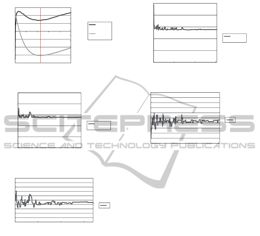
Figure 1 shows the relation between ε, correlation
coefficient and MSE. As shown in Fig.1, MSE be-
came minimal when we set ε to 0.42. At this time, the
correlation coefficient also became almost minimal.
SimulatedAnnealingbasedParameterOptimizationofTime-frequencye-filterUtilizingCorrelationCoefficient
239

2.5
3.0
3.5
4.0
4.5
5.0
0 1
0
0.1
0.2
0.3
0 0.2 0.4 0.6 0.8 1
Correlation
coefficient
MSE
0
0.5
1.0
1.5
2.0
-0.4
-0.3
-0.2
-
0
.
1
MSE minimal
[×10
-4
]
Correlation coefficient
MSE
ε
Figure 1: Relation between ε, correlation coefficient and
MSE.
0.1
0.15
0.2
0.25
Correlation
coefficient
0
0.05
0 100 200 300
Iteration counts
coefficient
Correlation coefficient
(a) Relation between iteration counts and correlation
coefficient.
0 3
0.4
0.5
0.6
0.7
0.8
0.9
1
ε
0
0.1
0.2
0
.
3
0 100 200 300
Iteration counts
ε
(b) Relation between iteration counts and ε.
Figure 2: Transition of correlation coefficient and ε when
we set the initial ε to 0.49.
Figure 2 shows the transition of correlation coef-
ficient and ε when we set the initial ε to 0.49, that
was obtained by Eq.14. As shown in Fig.2, we can
obtain the adequate ε utilizing the proposed method
automatically.
To show the robustness for changing the initial ε,
we conducted the experiments using the different ini-
tial ε. Figures 3 and 4 show the transition of corre-
lation coefficient and ε when we set the initial ε to
0.1 and 0.9, respectively. As shown in Figs.3 and 4,
we can obtain the adequate parameter of ε utilizing
the proposed method even when the initial ε is much
larger or smaller than the optimal ε.
0.1
0.15
0.2
0.25
Correlation
coefficient
0
0.05
0 100 200 300
Iteration counts
coefficient
Correlation coefficient
(a) Relation between iteration counts and correlation
coefficient.
0 4
0.5
0.6
0.7
0.8
0.9
1
ε
0
0.1
0.2
0.3
0
.
4
0 100 200 300
Iteration counts
ε
(b) Relation between iteration counts and ε.
Figure 3: Transition of correlation coefficient and ε when
we set the initial ε to 0.1.
5 CONCLUSIONS
In this paper, we employed the correlation coefficient
of the filter output and the difference between the in-
put and the filter output as the evaluation function of
the parameter setting of TF ε-filter. We also proposed
a simulated annealing based algorithm to determine
the parameter of TF ε-filter automatically. The ex-
perimental results show that we can automatically de-
termine the adequate parameters of TF ε-filter by uti-
lizing our method. As the proposed method only as-
sumes the decorrelation of the signal and noise, it is
expected that the application range of the proposed
method is large. Although we only have the single-
channel noisy signal, our method enables us to obtain
an adequate ε parameter automatically. The proposed
method does not require an estimation of the noise
in advance. The features will help us to use TF ε-
filter in a practical situation. To handle nonstation-
ary noise, we need to change ε adaptively depending
on the noise. Hence, we aim to improve our method
to solve this problem. For future studies, we would
like to evaluate robustness when changing the win-
dow size of the TF ε-filter. We also would like to de-
termine all parameters in TF ε-filter, that is, not only
SIGMAP2012-InternationalConferenceonSignalProcessingandMultimediaApplications
240

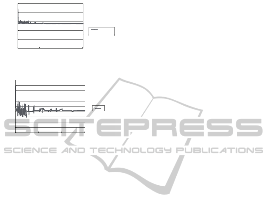
0.1
0.15
0.2
0.25
Correlation
coe
ffi
c
i
e
n
t
0
0.05
0 200 400 600
Iteration counts
coe c e t
Correlation coefficient
(a) Relation between iteration counts and correlation
coefficient.
0 4
0.5
0.6
0.7
0.8
0.9
1
ε
0
0.1
0.2
0.3
0
.4
0 200 400 600
Iteration counts
ε
(b) Relation between iteration counts and ε.
Figure 4: Transition of correlation coefficient and ε when
we set the initial ε to 0.9.
the ε value but also the window size adequately based
on automatic control.
ACKNOWLEDGEMENTS
This research was supported by Special Coordina-
tion Funds for Promoting Science and Technology,
by Japan Prize Foundation, NS promotion foundation
for science of perception and Foundation for the Fu-
sion Of Science and Technology, by Special Coordi-
nation Funds for Promoting Science and Technology,
and by the Ministry of Education, Science, Sports
and Culture, Grant-in-Aid for Young Scientists (B),
22700186, 2010. This research was also supported
by the CREST project “Foundation of technology
supporting the creation of digital media contents” of
JST, and by the Global-COE Program,“Global Robot
Academia”, Waseda University.
REFERENCES
Abe, T., Matsumoto, M., and Hashimoto, S. (2007). Noise
reduction combining time-domain ε-filter and time-
frequency ε-filter. In J. of the Acoust. Soc. America.,
volume 122, pages 2697–2705.
Abe, T., Matsumoto, M., and Hashimoto, S. (2009). Pa-
rameter optimization in time-frequency -filter based
on correlation coefficient. In Proc. of International
conference on signal processing and multimedia ap-
plications (SIGMAP2009), pages 107–111.
Boll, S. F. (1979). Suppression of acoustic noise in speech
using spectral subtraction. In IEEE Trans. Acoust.
Speech Signal Process., volume ASSP-27, pages 113–
120.
Daniel, P., Ellis, W., and Weiss., R. (2006). Model-based
monaural source separation using a vector-quantized
phase-vocoder representation. In Proc. IEEE Int’l
Conf. on Acoustics, Speech, and Signal Process. 2006.
Fujimoto, M. and Ariki, Y. (2002). Speech recognition un-
der noisy environments using speech signal estimation
method based on kalman filter. In IEICE Trans. Infor-
mation and Systems, volume J85-D-II, pages 1–11.
Harashima, H., Odajima, K., Shishikui, Y., and Miyakawa,
H. (1982). ε-separating nonlinear digital filter and its
applications. In IEICE trans on Fundamentals., vol-
ume J65-A, pages 297–303.
Kalman, R. E. (1960). A new approach to linear filtering
and prediction problems. In Trans. of the ASME, vol-
ume 82, pages 35–45.
Lim, J. S. (1978). Evaluation of a correlation subtraction
method for enhancing speech degraded by additive
white noise. In IEEE Trans. Acoust. Speech Signal
Process., volume ASSP-26, pages 471–472.
Lim, J. S., Oppenheim, A. V., and Braida, L. D. (1978).
Evaluation of an adaptive comb filtering method for
enhancing speech degraded by white noise addition.
In IEEE Trans. on Acoust. Speech Signal Process.,
volume ASSP-26, pages 419–423.
SimulatedAnnealingbasedParameterOptimizationofTime-frequencye-filterUtilizingCorrelationCoefficient
241