
Model Selection and Stability in Spectral Clustering
Zeev Volkovich and Renata Avros
Ort Braude College of Engineering, Software Engineering Department, Karmiel, Israel
K
eywords:
Spectral Clustering, Model Selection.
Abstract:
An open problem in spectral clustering concerning of finding automatically the number of clusters is studied.
We generalize the method for the scale parameter selecting offered in the Ng-Jordan-Weiss (NJW) algorithm
and reveal a connection with the distance learning methodology. Values of the scaling parameter estimated via
clustering of samples drawn are considered as a cluster stability attitude such that the clusters quantity corre-
sponding to the most concentrated distribution is accepted as true number of clusters. Numerical experiments
provided demonstrate high potential ability of the offered method.
1 INTRODUCTION
The recent decades, have seen numerous applications
of graph eigenvalues in many areas of combinatorial
optimization (Chung, 1997), (Mohar, 1997), (Spiel-
man, 2012). Spectral clustering methods became very
popular in the 21
th
century following Shi and Malik
(Shi and Malik, 2000) and Ng, Jordan and Weiss (Ng
et al., 2001). Over the last decade, various spectral
clustering algorithms have been developed and ap-
plied to computer vision (Ng et al., 2001), (Shi and
Malik, 2000), (Yu and Shi, 2003), network science
(Fortunato, 2010), (White and Smyth, 2005), biomet-
rics (Wechsler, 2010), text mining (Liu et al., 2009),
natural language processing (Dasgupta and Ng, 2009)
and other areas. We note that spectral clustering meth-
ods have been found equivalent to kernel k-means
(Dhillon et al., 2004), (Kulis et al., 2005) as well
as to nonnegative matrix factorization (Ding et al.,
2005). For surveys on spectral clustering, see (Nasci-
mento and Carvalho, 2011), (Luxburg, 2007), (Filip-
pone et al., 2008).
The main idea is to use eigenvectors of the Lapla-
cian matrix, based on an affinity (similarity) func-
tion over the data. The Laplacian is a positive semi-
definite matrix whose eigenvalues are nonnegative re-
als. It is well-known that the smallest eigenvalue of
the Laplacian is 0, and it corresponds to an eigen-
vector with all entries equal. Moreover, viewing the
data similarity function as an adjacency matrix of a
graph, the multiplicity of the 0 eigenvalue is the num-
ber of connected components (Mohar, 1997). While
in clustering problems the corresponding graph is typ-
ically connected, we partition the data into k clusters
using the k eigenvectors corresponding to the k small-
est eigenvalues. These would either be the k smallest
eigenvectors or the k largest eigenvectors, depending
on the Laplacian version being used. For example, a
simple way of partitioning the data into two clusters
would be considering the second eigenvector as an in-
dicator vector, assigning items with positive coordi-
nate values into one cluster, and items with negative
coordinate values to another cluster.
Spectral clustering algorithms have several signif-
icant advantages. First, they do not make any assump-
tions on the clusters, which allows flexibility in dis-
covering various partitions (unlike the k-means algo-
rithm, for example, which assumes that the clusters
are spherical). Second, they rely on basic linear alge-
bra operations. And finally, while spectral clustering
methods can be costly for large and “dense” data sets,
they are particularly efficient when the Laplacian ma-
trix is sparse (i.e., when many pairs of points are of
zero affinity). Spectral methods can also serve in di-
mensionality reduction for high-dimensional data sets
(the new dimension being the number of clusters k).
Note, that the problem to determine the optimal
(“true”) number of groups for a given data set is very
crucial in cluster analysis. This task arising in many
applications. As usual, the clustering solutions, ob-
tained for several numbers of clusters are compared
according to the chosen criteria. The sought number
yields the optimal quality in accordance with the cho-
sen rule. The problem may have more than one solu-
tion and is known as an “ill posed” (Jain and Dubes,
1988) and (Gordon, 1999). For instance, an answer
here can depend on the scale in which the data is mea-
sured. Many approaches were proposed to solve this
25
Volkovich Z. and Avros R..
Model Selection and Stability in Spectral Clustering .
DOI: 10.5220/0004132700250034
In Proceedings of the International Conference on Knowledge Discovery and Information Retrieval (KDIR-2012), pages 25-34
ISBN: 978-989-8565-29-7
Copyright
c
2012 SCITEPRESS (Science and Technology Publications, Lda.)

problem, yet none has been accepted as superior so
far.
From a geometrical point of view, cluster val-
idation has been studied in the following papers:
Dunn (Dunn, 1974), Hubert and Schultz (Hubert
and Schultz, 1974), Calinski-Harabasz (Calinski
and Harabasz, 1974), Hartigan (Hartigan, 1985),
Krzanowski -Lai (Krzanowski and Lai, 1985), Sugar-
James (Sugar and James, 2003), Gordon (Gordon,
1994), Milligan and Cooper (Milligan and Cooper,
1985) and Tibshirani, Walter and Hastie (Tibshirani
et al., 2001) (the Gap Statistic method). Here, the
so-called “elbow” criterion plays a central role in the
indication of the “true” number of clusters.
In the papers Volkovich, Barzily and Morozensky
(Volkovich et al., 2008), Barzily, Volkovich, Akteke-
Ozturk and Weber (Barzily et al., 2009), Toledano-
Kitai, Avros and Volkovich (Toledano-Kitai et al.,
2011), methods using the goodness of fit concepts are
suggested. Here, the source cluster distributions are
constructed based on a model designed to represent
well-mixed samples within the clusters.
Another very common, in this area, methodology
employs the stability concepts. Apparently, Jain and
Moreau (Jain and Moreau, 1987) were the first to pro-
pose such a point of view in the cluster validation
thematic and used the dispersions of empirical dis-
tributions of the cluster object function as a stabil-
ity measure. Following this perception, differences
between solutions obtained via rerunning a cluster-
ing algorithm on the same datum evaluate the parti-
tions stability. Hence, the number of clusters mini-
mizing partitions’ changeability is used to assess the
“true” number of clusters. In papers of Levine and
Domany (Levine and Domany, 2001), Ben-Hur, Elis-
seeff and Guyon (Ben-Hur et al., 2002), Ben-Hur and
Guyon (Ben-Hur and Guyon, 2003) and Dudoit and
Fridlyand (Dudoit and Fridlyand, 2002) (the CLEST
method), stability criteria are understood to be the
fraction of times that pairs of elements maintain the
same membership under reruns of the clustering al-
gorithm. Mufti, Bertrand, and El Moubarki (Mufti
et al., 2005) exploit Loevinger’s measure of isolation
to determine a stability function.
In this paper we offer a new approach to an open
problem in spectral clustering which concerns auto-
matically finding the number of clusters. Our ap-
proach is based on the stability concept. Here we
generalize the method for the scale parameter select-
ing offered in the Ng-Jordan-Weiss (NJW) algorithm
and reveal a connection with the distance learning
methodology. Values of the scaling parameter, es-
timated via clustering of the drawn samples for the
number of clusters allocated in a given area, are con-
sidered as a cluster stability attitude such that the
preferred number of clusters corresponds to the most
concentrated empirical distribution of the parameter.
Provided numerical experiments demonstrate high
potential ability of the offered method. The rest of
the paper is organized in the following way. Section
2 is devoted to statement of the base facts of cluster
analyzes used and to a discussion of the scale param-
eter selection approaches. In section 3 we propose an
application of the offered methodology to the cluster
validation problem. Section 4 is devoted to the nu-
merical experiments provided.
2 CLUSTERING
We consider a finite subset X = {x
1
,...,x
n
} of the
Euclidean space R
d
. A partition of the set X into k
clusters is a collection of k non-empty of its subsets
Π
k
= {π
1
,...,π
k
} satistiyng the conditions:
k
[
i=1
π
i
= X,
π
i
∩ π
j
= ∅ if i 6= j.
The partition’s elements are named clusters.
Two partitions are identical if and only if every clus-
ter in the first partition is also presented in the second
one and vice versa. In other words, both partitions
have the same clusters up to a permutation. In cluster
analysis a partition is chosen so that a given quality
Q(Π
k
) =
k
∑
i=1
q(π
i
)
is optimized for some real valued function q whose
domain is the set of subsets of X. The function q is
a distance-like function and, commonly, it is not re-
quired to be positive or to satisfy the triangle inequal-
ity. In case of the hard clustering the underlying dis-
tribution of X is assumed to be represented in the form
µ
X
=
k
∑
i=1
p
i
η
i
,
where p
i
, i = 1, .., k are the clusters’ probabilities and
η
i
, i = 1,..,k are the clusters’ distributions. Note, that
this supposition is widespread in clustering, pattern
recognition and multivariate density estimation (see,
for example (McLachlan and Peel, 2000)). Partic-
ularly, the most prevalent Gaussian model considers
distributions η
i
having densities
f
i
(x) = φ(x|m
i
,Γ
i
), i = 1,...,k,
where φ(x|m
i
,Γ
i
) denotes the Gaussian density with
mean vector m
i
and covariance matrix Γ
i
. Usually,
the mixture parameters
KDIR2012-InternationalConferenceonKnowledgeDiscoveryandInformationRetrieval
26

θ = (p
i
,m
i
,Γ
i
), i = 1,...,k
are estimated in this case by maximizing the likeli-
hood
L(θ|x
1
,...,x
n
) =
n
∑
j=1
ln
k
∑
i=1
p
i
φ(x
j
|m
i
,Γ
i
)
!
. (1)
The most common procedure for maximum likeli-
hood clustering solution is the EM algorithm (see, for
example (McLachlan and Peel, 2000)). The EM al-
gorithm provides, in many cases, meaningful results.
However, the algorithm often converges slowly and
has a strong dependence on its starting position. One
of the important EM related algorithms is a Classifica-
tion EM algorithm (CEM) introduced by Celeux and
Govaert in (Celeux and Govaert, 1992). CEM max-
imizes the Classification Likelihood criterion which
is different from the Maximum Likelihood criterion
(1). In fact, it does not yield maximum likelihood es-
timates and can lead to inconsistent values (see, for
example (McLachlan and Peel, 2000), section 2.21).
The k-means approach has been introduced in
(Forgy, 1965) and in (MacQueen, 1967). It provides
the clusters which approximately minimize the sum
of the items’ squared Euclidean distances from clus-
ter centers, which are called centroids. The algorithm
generates linear boundaries among clusters. Celeux
and Govaert (Celeux and Govaert, 1992) showed that,
in the case of the Gaussian mixture model, this proce-
dure actually assumes that all mixture proportions are
equal
p
1
= p
2
= ... = p
k
;
and the covariance matrix is of the form:
Γ
i
= σ
2
I, i = 1,...,k,
where I is the identity matrix of order d and σ
2
is
an unknown parameter. In other words, the k-means
algorithm is, evidently, a particular case of the CEM
algorithm.
Spectral clustering skills commonly leverage the
spectrum of a given similarity matrix in order to
perform dimensionality reduction for clustering in
fewer dimensions. Note, that there is a large family
of possible algorithms based on the spectral cluster-
ing methodology (see, for example (Nascimento and
Carvalho, 2011), (Luxburg, 2007), (Filippone et al.,
2008)).
Here, we concentrate on a relatively simple tech-
nique offered in (Ng et al., 2001) in order to demon-
strate the ability of the proposed approach.
Algorithm 2.1. Spectral Clustering(X,k,σ)(NJW)
Input
• X - the data to be clustered;
• k - number of clusters;
• σ - the scaling parameter.
Output
Π
k, σ
(X)- a partition of X into k clusters depending
on σ.
====================
• Construct the affinity matrix A(σ
2
)
{a
ij
(σ
2
)} =
exp
−
k
x
i
−x
j
k
2
2σ
2
if i 6= j,
0 otherwise
• Introduce L = D
−
1
2
A(σ
2
)D
−
1
2
where D is the di-
agonal matrix whose (i,i)-element is the sum of
A′s i-th row.
(Note, that the acceptable point of view proposes
to deal with the Laplacian I − L. However, the
authors (Ng et al., 2001) prefer to work with L and
only to change the eigenvalues (from A to I − A)
without any changing of the eigenvectors.)
• Compute z
1
,z
2
,...,z
k
, the k largest eigenvectors of
L (chosen to be orthogonal to each other in the
case of repeated eigenvalues);
• Create the matrix Z = {z
1
,z
2
,...,z
k
} ∈ R
n×k
by
joining the eigenvectors as consequent columns;
• Compute the matrixY from Z by normalizing each
of Z’s rows to have a unit length;
• Cluster the rows of Y into k clusters via K-means
or any other algorithm (that attempts to minimize
distortion) to obtain a partition Π
k, σ
(Y);
• Assign each point x
i
according to the cluster that
was assigned to the row i in the obtained partition.
Note, that there is a one to one correspondence be-
tween the partitions Π
k, σ
(X) and Π
k, σ
(Y). The mag-
nitude parameter σ
2
represents the increasing rate of
the affinity of the distance function. This parameter
plays a very important role in the clustering process
and can be naturally reached as the outcome of an
optimization problem intended to find the best pos-
sible partition configuration. An appropriate meta al-
gorithm could be presented in the following form.
Algorithm 2.2. Self-Learning Spectral Clustering
(X, k,F)
Input
• X - the data to be clustered;
• k - number of clusters;
ModelSelectionandStabilityinSpectralClustering
27

• F - cluster quality function to be minimized.
Output
• σ
∗
- an optimal value of the the scaling parame-
ter;
• Π
k, σ
∗
(X)−a partition of X into k clusters corre-
sponding to σ
∗
.
====================
Return
σ
∗
= argmin
σ
(F(Π
k, σ
(X) =
= Spectral Clustering(X,k,σ))).
When σ
2
is described as a human-specified pa-
rameter which is selected to form the “tight” k clusters
on the surface of the k-sphere. Consequently, it is rec-
ommended to search over σ
2
and to take the value that
gives the tightest (smallest distortion) clusters of the
set Y. This procedure can be generalized. Here
F
1
(Π
k, σ
(X)) =
1
|Y|
k
∑
i=1
∑
y∈π
i
ky− r
i
k
2
, (2)
where r
i
, i = 1, ..., k are cluster’s centroids.
Other functions of this kind can be found in the
framework of the distance learning methodology. In
what follows, it is presumed that the degree of simi-
larity between pairs of elements of data collection is
known:
S : {(x
i
,x
j
); if x
i
and x
j
are similar
(belong to the same cluster)}
and
D : {(x
i
,x
j
); if x
i
and x
j
are not similar
(belong to dif f erent clusters)}
the goal is to learn a distance metric d(x,y) such that
all “similar” data points are kept in the same clus-
ter, (i.e., close to each other) while distinguishing the
“dissimilar” data points. To this end, we define a dis-
tance metric in the form:
d
2
C
(x,y) = k x − yk
2
A
= (x− y)
T
·C ·(x− y),
where C is a positive semi-definite matrix, C ≻ 0
which is learned. We can formulate a constrained
optimization problem where we aim to minimize the
sum of similar distances concerning pairs in S while
maximizing the sum of dissimilar distances related to
pairs in D in the following way:
min
C
∑
(
x
i
,x
j
)
∈S
x
i
− x
j
2
C
s.t.
∑
(
x
i
,x
j
)
∈D
x
i
− x
j
2
C
≥ 1, C ≻ 0
If we suppose that the purported metric matrix is di-
agonal then minimizing the function is equivalent to
solving the stated optimization problem (Xing et al.,
2002) up to a multiplication of C by a positive con-
stant. So, the second quality function can be offered
as
F
2
(Π
k, σ
(X)) =
∑
(
x
i
,x
j
)
∈S,i6= j
y
i
− y
j
2
− (3)
−log
∑
(
x
i
,x
j
)
∈D
y
i
− y
j
.
Finally, in the spirit of the Fisher’s linear discriminant
analysis we can consider the function:
F
3
(Π
k, σ
(X)) =
∑
(
x
i
,x
j
)
∈S,i6= j
y
i
− y
j
2
∑
(
x
i
,x
j
)
∈D
y
i
− y
j
2
. (4)
3 AN APPLICATION TO THE
CLUSTER VALIDATION
PROBLEM
In this section we discuss an application of the of-
fered methodology to the cluster validation problem.
We suggest that these values should be learned from
samples clustered for several clusters quantities such
that the most stable behaviour of the parameter is ex-
hibited when the cluster structure is the most stable.
In our case, it means that the number of clusters is
chosen by the best possible way. The drawbacks of
the used algorithm together with the complexity of the
dataset structure add to the uncertainty of the process
outcome. To overcome this ambiguity, a sufficient
amount of data has to be involved. This is achieved
by drawing many samples and constructing an empir-
ical distribution of the scaling parameter values. The
most concentrated distribution corresponds to the ap-
propriate number of clusters.
Algorithm 3.1. Spectral Clustering Validation
(X, K,F, J, m, Ind)
Input
• X - the data to be clustered;
• K - maximal number of clusters to be tested;
• F - cluster quality function to be minimized;
• J- number of samples to be drawn;
• m - size of samples to be to be drawn;
• Ind - concentration index.
KDIR2012-InternationalConferenceonKnowledgeDiscoveryandInformationRetrieval
28
Output
• k
∗
− an estimated number of clusters in the
dataset.
====================
• For k = 2 to K do
• For j = 1 to J do
• S = sample(X,m);
• σ
j
=Self-Learning Spectral Cluster-
ing(X, k,F);
• end For j
• Compute C
k
= Ind{σ
1
,...,σ
J
}
• end For k
• The “true” number of clusters - k
∗
is chosen ac-
cording to the most concentrated distribution indi-
cated by an appropriate value of C
k
, k = 2,...,K.
3.1 Remarks Concerning the Algorithm
Here, sample (X,m) denotes a procedure of drawing
a sample of size m from the population X without rep-
etitions. Concentration indexes can be provided in
several ways. The most widespread instrument used
for the evaluation of a distribution’s concentration is
the standard deviation. However, it is sensitive to out-
liers and can be principally dependent, in our situa-
tion, on the number of clusters examined. To counter-
balance this reliance, the values have be normalized.
Unfortunately, it has been specified in the clustering
literature that the standard “correct” strategy, for nor-
malization and scaling, does not exist (see, for exam-
ple (Roth et al., 2004) and (Tibshirani et al., 2001)).
We use the coefficient of variation (CV) which is de-
fined as the ratio of the sample standard deviation
to the sample mean. For comparison between arrays
with different units this value is preferred to the stan-
dard deviation because it is a dimensionless number.
4 NUMERICAL EXPERIMENTS
We exemplify the described approach by means of
various numerical experiments on synthetic and real
datasets provided for the three functions mentioned
in 2-4. We choose K = 7 in all tests and perform 10
trials for each experiment. The results are presented
via the error-bar plots of the coefficient of variation
within the trials.
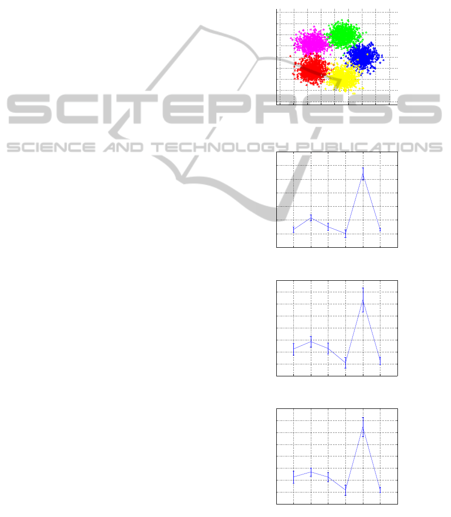
4.1 Synthetic Data
The first example consists of a mixture of 5 two-
dimensional Gaussian distributions with independent
coordinates with the same standard deviation σ =
0.25. The components means are placed on the unit
circle with the angular neighboring distance 2π/5.
The dataset contains (denoted as G5) 4000 items. The
scatterplot of this data is presented in the next figure
−2 −1.5 −1 −0.5 0 0.5 1 1.5 2
−2
−1.5
−1
−0.5
0
0.5
1
1.5
2
Figure 1: Scatterplot of the Gaussian dataset.
We set here J = 100 and m = 400.
1 2 3 4 5 6 7 8
0.2
0.4
0.6
0.8
1
1.2
1.4
1.6
Figure 2: CV for the G5 dataset using F1 function.
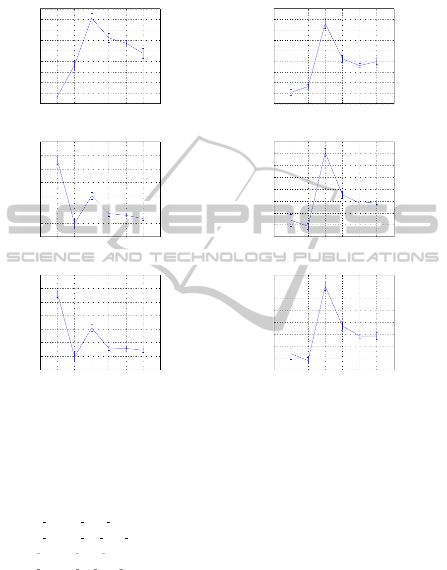
1 2 3 4 5 6 7 8
0.4
0.5
0.6
0.7
0.8
0.9
1
1.1
Figure 3: CV for the G5 dataset using F2 function.
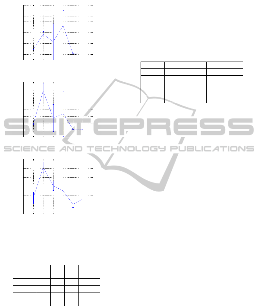
1 2 3 4 5 6 7 8
0.4
0.5
0.6
0.7
0.8
0.9
1
1.1
Figure 4: CV for the G5 dataset using F3 function.
ModelSelectionandStabilityinSpectralClustering
29
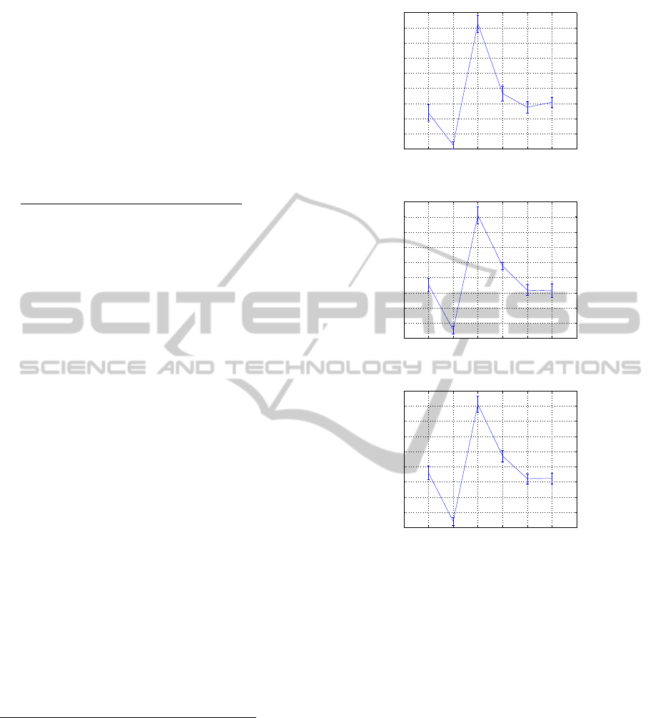
The CV index demonstrates approximately the
same performance for all object functions hinting to
a 5 or 7 clusters structure. However, the bars do not
overlap only in the first case where a 5 cluster parti-
tion is properly indicated.
4.2 Real-world Data
4.2.1 Three Texts Collection
The first real dataset is chosen from the text collection
http : //ftp.cs.cornell.edu/pub/smart/.
This set (denoted as T3) includes the following
three text collections:
• DC0–Medlars Collection (1033 medical ab-
stracts);
• DC1–CISI Collection (1460 information science
abstracts);
• DC2–Cranfield Collection (1400 aerodynamics
abstracts).
This dataset was considered in many works
(Dhillon and Modha, 2001), (Kogan et al., 2003a),
(Kogan et al., 2003b), (Kogan et al., 2003c) and
(Volkovich et al., 2004)). Usually, following the well-
known “bag of words” approach, 600 “best” terms
were selected (see, (Dhillon et al., 2003) for term se-
lection details). So, the dataset was mapped into Eu-
clidean spaces with dimensions 600. A dimension re-
duction is providedby the Principal Component Anal-
ysis (PCA). The considered dataset is recognized to
be well- separated by means of the two leading prin-
cipal components. We use this data representation in
our experiments. The results presented in Fig. 5-7
for m = J = 100 show that the number of clusters was
properly determined for all functions F.
4.2.2 Iris Flower Dataset
Another real dataset chosen is the well-known Iris
flower dataset or Fisher’s Iris dataset available, for ex-
ample, at
http : //archive.ics.uci.edu/ml/datasets/Iris.
The collection includes 50 samples from each of
three species of Iris flowers:
• I. setosa;
• I. virginica;
• I. versicolor.
These species compose three clusters situated in a
manner that one cluster is linearly separable from the
others, but the other two are not. This dataset was an-
alyzed in many papers. A two cluster structure was
detected in (Roth et al., 2002). Here, we selected 100
1 2 3 4 5 6 7 8
0.1
0.2
0.3
0.4
0.5
0.6
0.7
0.8
0.9
1
Figure 5: CV for the T3, 600 terms, using F1 function.
1 2 3 4 5 6 7 8
0.1
0.2
0.3
0.4
0.5
0.6
0.7
0.8
0.9
1
Figure 6: CV for the T3, 600 terms,using F2 function.
1 2 3 4 5 6 7 8
0.1
0.2
0.3
0.4
0.5
0.6
0.7
0.8
0.9
1
Figure 7: CV for the T3, 600 terms, using F3 function.
samples of size 140 for each tested number of clus-
ters. As it can be seen, the “true” number of clusters
has been successfully found for the F2 and F3 objec-
tive functions. The experiments with F1 offer a two
clusters configuration.
4.2.3 The Wine Recognition Dataset
The last real dataset contains 178 results of a chemical
analysis of three different types (cultivates) of wine
given by their 13 ingredients. This collection is avail-
able at
http://archive.ics.uci.edu/ml/machine-learning-
databases/wine. This data collection is relatively
small however it exhibits a high dimension. The
parameters in use were J = 100 and m = 100. Fig. 4
demonstrates undoubtedly that for F2 and F3 the true
number of clusters is revealed, however F1 detects a
wrong structure.
KDIR2012-InternationalConferenceonKnowledgeDiscoveryandInformationRetrieval
30
1 2 3 4 5 6 7 8
0
0.1
0.2
0.3
0.4
0.5
0.6
0.7
0.8
0.9
Figure 8: CV for the Iris dataset using F1 function.
1 2 3 4 5 6 7 8
0.2
0.4
0.6
0.8
1
1.2
1.4
1.6
Figure 9: CV for the Iris dataset using F2 function.
1 2 3 4 5 6 7 8
0.2
0.4
0.6
0.8
1
1.2
1.4
1.6
Figure 10: CV for the Iris dataset using F3 function.
4.2.4 The Glass Dataset
This dataset is taken from the UC Irvine Machine
Learning Repository collection. (http://archive.ics.
uci.edu/ml/index.html). The study of classification of
glass types was motivated by criminology investiga-
tion.The glass found at the place of a crime, can be
used as evidence. Number of Instances: 214. Num-
ber of Attributes: 9. Type of glass: (class attribute)
• building windows float processed;
• building windows non float processed;
• vehicle windows float processed;
• vehicle windows non float processed
(notpresented);
• containers;
• tableware;
• headlamps.
1 2 3 4 5 6 7 8
0
0.1
0.2
0.3
0.4
0.5
0.6
0.7
0.8
0.9
Figure 11: CV for the Wine dataset using F1 function.
1 2 3 4 5 6 7 8
0.1
0.2
0.3
0.4
0.5
0.6
0.7
0.8
0.9
Figure 12: CV for the Wine dataset using F2 function.
1 2 3 4 5 6 7 8
0.1
0.2
0.3
0.4
0.5
0.6
0.7
0.8
0.9
Figure 13: CV for the Wine dataset using F3 function.
Fig. 14-16 demonstrate outcomes obtained for
J = 100. Note, that this relatively small dataset pos-
sess a comparatively large dimension and a signifi-
cantly larger, in comparison with previous collection,
suggested number of clusters. To eliminate the influ-
ence of the sample size on the clustering solutions we
draw samples with growing sizes m = max((k − 1) ∗
40,214). The minimal value depicted in the graph
corresponding to the F3 function is 6, however the
bars of ”2” and ”6” overlap. Since the index behav-
ior is more stable once the number of clusters is 6,
this value is accepted as the true number of clusters.
Other function do not success in determining the true
number of clusters.
4.2.5 Comparison of the Partition Quality
Function used
Table 1 summarizes the results of the numerical ex-
periments provided. As can be seen, the functions F2
ModelSelectionandStabilityinSpectralClustering
31
1 2 3 4 5 6 7 8
−1
0
1
2
3
4
5
6
7
8
9
Figure 14: CV for the Glass dataset using F1 function.
1 2 3 4 5 6 7 8
−1
0
1
2
3
4
5
6
7
Figure 15: CV for the Glass dataset using F2 function.
1 2 3 4 5 6 7 8
0.4
0.5
0.6
0.7
0.8
0.9
1
Figure 16: CV for the Glass dataset using F3 function.
and F3, introduced in this paper, subsume the previ-
ously offered function F1.
Table 1: Comparison of the partition quality function used.
Dataset F1 F2 F3 TRUE
G5 5 5,7 5,7 5
T3 3 3 3 3
Iris 2 3 3 3
Wine 2 3 3 3
Glass 7 7 6 6
4.2.6 Comparison with Other Methods
In addition to an experimental study of the presented
cluster quality functions, we also provide a compari-
son of our method with several other cluster valida-
tion approaches. In particular, we evaluate the re-
sults obtained by the Calinski and Harabasz index
(CH) (Calinski and Harabasz, 1974), the Krzanowski
and Lai index (KL) (Krzanowski and Lai, 1985), the
Sugar and James index (SJ) (Sugar and James, 2003),
the GAP-index (Tibshirani et al., 2001) and the Clest-
index (Dudoit and Fridlyand, 2002). Our method suc-
ceeds quite well in the comparison in case ones an
appropriate quality function was chosen.
Table 2: Comparison with other methods.
Dataset CH KL SJ Gap Clest
G5 5 5 5 3 6
T3 3 3 1 3 2
Iris 2 2 4 7 7
Wine 3 2 3 6 1
Glass 2 2 2 6 3
5 CONCLUSIONS AND FUTURE
WORK
In this paper a new approach to determine the number
of the groups in spectral clustering was presented. An
empirical distribution of the scaling parameter, found
resting upon samples clusterization, is considered as
a new cluster stability feature. We analyze three cost
functions which can be used in a self-tuning version
of a spectral clustering algorithm. In the future re-
search we plan to generalize our method to the Lo-
cal Scaling methodology (Zelnik-manor and Perona,
2004) and compare the obtained outcomes. Another
research direction can consist of a study of the model
behavior when the number of clusters is suggested to
be relatively big. An essential ingredient of each re-
sampling cluster validation approach is the selection
of the parameters values in an implementation. It is
difficult to treat this task from a theoretical point of
view (see, e.g. (Dudoit and Fridlyand, 2002), (Roth
et al., 2004) and (Levine and Domany,2001)). We are
going to investigate this matter in our future papers.
REFERENCES
Barzily, Z., Volkovich, Z., Akteko-Ozturk, B., and We-
ber, G.-W. (2009). On a minimal spanning tree ap-
proach in the cluster validation problem. Informatica,
20(2):187–202.
Ben-Hur, A., Elisseeff, A., and Guyon, I. (2002). A stabil-
ity based method for discovering structure in clustered
data. In Pacific Symposium on Biocomputing, pages
6–17.
Ben-Hur, A. and Guyon, I. (2003). Detecting stable clusters
using principal component analysis. In Brownstein,
M. and Khodursky, A., editors, Methods in Molecular
Biology, pages 159–182. Humana press.
KDIR2012-InternationalConferenceonKnowledgeDiscoveryandInformationRetrieval
32

Calinski, R. and Harabasz, J. (1974). A dendrite method for
cluster analysis. Communications in Statistics, 3:1–
27.
Celeux, G. and Govaert, G. (1992). A classification EM
algorithm for clustering and two stochastic versions.
Computational Statistics and Data Analysis, 14:315–
332.
Chung, F. R. K. (1997). Spectral Graph Theory. AMS
Press, Providence, R.I.
Dasgupta, S. and Ng, V. (2009). Mine the easy, classify the
hard: a semi-supervised approach to automatic senti-
ment classification. In ACL-IJCNLP 2009: Proceed-
ings of the Main Conference, pages 701–709.
Dhillon, I., Kogan, J., and Nicholas, C. (2003). Feature
selection and document clustering. In Berry, M., ed-
itor, A Comprehensive Survey of Text Mining, pages
73–100. Springer, Berlin Heildelberg New York.
Dhillon, I. S., Guan, Y., and Kulis, B. (2004). Kernel k-
means, spectral clustering and normalized cuts. In
Proceedings of the Tenth ACM SIGKDD International
Conference on Knowledge Discovery and Data Min-
ing (KDD), pages 551–556.
Dhillon, I. S. and Modha, D. S. (2001). Concept decom-
positions for large sparse text data using clustering.
Machine Learning, 42(1):143–175. Also appears as
IBM Research Report RJ 10147, July 1999.
Ding, C., He, X., and Simon, H. D. (2005). On the equiv-
alence of nonnegative matrix factorization and spec-
tral clustering. In Proceedings of the fifth SIAM inter-
national conference on data mining, volume 4, pages
606–610.
Dudoit, S. and Fridlyand, J. (2002). A prediction-based re-
sampling method for estimating the number of clus-
ters in a dataset. Genome Biol., 3(7).
Dunn, J. C. (1974). Well Separated Clusters and Optimal
Fuzzy Partitions. Journal on Cybernetics, 4:95–104.
Filippone, M., Camastra, F., Masulli, F., and Rovetta, S.
(2008). A survey of kernel and spectral methods for
clustering. Pattern Recognition, 41(1):176–190.
Forgy, E. W. (1965). Cluster analysis of multivariate data
- efficiency vs interpretability of classifications. Bio-
metrics, 21(3):768–769.
Fortunato, S. (2010). Community detection in graphs. Phys.
Rep., 486(3-5):75–174.
Gordon, A. D.(1994). Identifying genuine clusters in a clas-
sification. Computational Statistics and Data Analy-
sis, 18:561–581.
Gordon, A. D. (1999). Classification. Chapman and Hall,
CRC, Boca Raton, FL.
Hartigan, J. A. (1985). Statistical theory in clustering. J.
Classification, 2:63–76.
Hubert, L. and Schultz, J. (1974). Quadratic assignment as
a general data-analysis strategy. Br. J. Math. Statist.
Psychol., 76:190–241.
Jain, A. and Dubes, R. (1988). Algorithms for Clustering
Data. Englewood Cliffs, Prentice-Hall, New Jersey.
Jain, A. K. and Moreau, J. V. (1987). Bootstrap technique in
cluster analysis. Pattern Recognition, 20(5):547–568.
Kogan, J., Nicholas, C., and Volkovich, V. (2003a). Text
mining with hybrid clustering schemes. In M.W.Berry
and Pottenger, W., editors, Proceedings of the Work-
shop on Text Mining (held in conjunction with the
Third SIAM International Conference on Data Min-
ing), pages 5–16.
Kogan, J., Nicholas, C., and Volkovich, V. (Novem-
ber/December 2003b). Text mining with information–
theoretical clustering. Computing in Science & Engi-
neering, pages 52–59.
Kogan, J., Teboulle, M., and Nicholas, C. (2003c). Opti-
mization approach to generating families of k–means
like algorithms. In Dhillon, I. and Kogan, J., editors,
Proceedings of the Workshop on Clustering High Di-
mensional Data and its Applications (held in conjunc-
tion with the Third SIAM International Conference on
Data Mining).
Krzanowski, W. and Lai, Y. (1985). A criterion for deter-
mining the number of groups in a dataset using sum
of squares clustering. Biometrics, 44:23–34.
Kulis, B., Basu, S., Dhillon, I., and Mooney, R. J. (2005).
Semi-supervised graph clustering: A kernel approach.
In Proceedings of the 22nd International Conference
on Machine Learning, pages 457–464, Bonn, Ger-
many.
Levine, E. and Domany, E. (2001). Resampling method
for unsupervised estimation of cluster validity. Neural
Computation, 13:2573–2593.
Liu, X., Yu, S., Moreau, Y., Moor, B. D., Glanzel, W., and
Janssens, F. A. L. (2009). Hybrid clustering of text
mining and bibliometrics applied to journal sets. In
SDM’09, pages 49–60.
Luxburg, U. V. (2007). A tutorial on spectral clustering.
Statistics and Computing, 17(4):395–416.
MacQueen, J. B. (1967). Some methods for classification
and analysis of multivariate observations. In Pro-
ceedings of 5-th Berkeley Symposium on Mathemat-
ical Statistics and Probability, volume 1, pages 281–
297. Berkeley, University of California Press.
McLachlan, G. J. and Peel, D. (2000). Finite Mixure Mod-
els. Wiley.
Milligan, G. and Cooper, M. (1985). An examination of
procedures for determining the number of clusters in
a data set. Psychometrika, 50:159–179.
Mohar, B. (1997). Some applications of Laplace eigen-
values of graphs. G. Hahn and G. Sabidussi (Eds.),
Graph Symmetry: Algebraic Methods and Applica-
tions, Springer.
Mufti, G. B., Bertrand, P., and Moubarki, E. (2005). Deter-
mining the number of groups from measures of cluster
validity. In Proceedings of ASMDA 2005, pages 404–
414.
Nascimento, M. and Carvalho, A. D. (2011). Spectral meth-
ods for graph clustering – a survey. European Journal
Of Operational Research, 2116(2):221–231.
Ng, A. Y., Jordan, M. I., and Weiss, Y. (2001). On spectral
clustering: analysis and an algorithm. In Advances
in Neural Information Processing Systems 14 (NIPS
2001), pages 849–856.
Roth, V., Lange, V., Braun, M., and J., B. (2002). A resam-
pling approach to cluster validation. In COMPSTAT,
available at http://www.cs.uni-bonn.De/
˜
braunm.
ModelSelectionandStabilityinSpectralClustering
33

Roth, V., Lange, V., Braun, M., and J., B. (2004). Stability-
based validation of clustering solutions. Neural Com-
putation, 16(6):1299 – 1323.
Shi, J. and Malik, J. (2000). Normalized cuts and image
segmentation. IEEE Transactions on Pattern Analysis
and Machine Intelligence, 22(8):888–905.
Spielman, D. A. (2012). Spectral graph theory. U. Nau-
mann and O. Schenk (Eds.), Combinatorial Scien-
tific Computing, Chapman & Hall/CRC Computa-
tional Science.
Sugar, C. and James, G. (2003). Finding the number of
clusters in a data set: An information theoretic ap-
proach. J. of the American Statistical Association,
98:750–763.
Tibshirani, R., Walther, G., and Hastie, T. (2001). Esti-
mating the number of clusters via the gap statistic. J.
Royal Statist. Soc. B, 63(2):411–423.
Toledano-Kitai, D., Avros, R., and Volkovich, Z. (2011). A
fractal dimension standpoint to the cluster validation
problem. International Journal of Pure and Applied
Mathematics, 68(2):233–252.
Volkovich, V., Kogan, J., and Nicholas, C. (2004). k–means
initialization by sampling large datasets. In Dhillon,
I. and Kogan, J., editors, Proceedings of the Workshop
on Clustering High Dimensional Data and its Appli-
cations (held in conjunction with SDM 2004), pages
17–22.
Volkovich, Z., Barzily, Z., and Morozensky, L. (2008). A
statistical model of cluster stability. Pattern Recogni-
tion, 41(7):2174–2188.
Wechsler, H. (2010). Intelligent biometric information
management. Intelligent Information Management,
2:499–511.
White, S. and Smyth, P. (2005). A spectral clustering ap-
proach to finding communities in graphs. In Proceed-
ings of the fifth SIAM international conference on data
mining, volume 119, pages 274–285. Society for In-
dustrial Mathematics.
Xing, E. P., Ng, A. Y., Jordan, M. I., and Russell, S. (2002).
Distance metric learning, with application to cluster-
ing with side-information. Advances in Neural In-
formation Processing Systems 15 (NIPS 2002), pages
505–512.
Yu, S. X. and Shi, J. (2003). Multiclass spectral clustering.
In Proceedings of the Ninth IEEE International Con-
ference on Computer Vision, volume 1, pages 313–
319.
Zelnik-manor, L. and Perona, P. (2004). Self-tuning spectral
clustering. In Advances in Neural Information Pro-
cessing Systems 17, pages 1601–1608. MIT Press.
KDIR2012-InternationalConferenceonKnowledgeDiscoveryandInformationRetrieval
34
