Some Empirical Evaluations of a Temperature Forecasting Module based

on Artiﬁcial Neural Networks for a Domotic Home Environment

F. Zamora-Mart

ınez, P. Romeu, J. Pardo and D. Tormo

Embedded Systems and Artiﬁcial Intelligence Group, Departamento de Ciencias F

ısicas, Matem

aticas y de la

Computaci

on, Escuela Superior de Ense

nanzas T

ecnicas (ESET), Universidad CEU Cardenal Herrera,

46115 Alfara del Patriarca, Valencia, Spain

Keywords:

Artiﬁcial Neural Networks, Temporal Series Forecasting, Domotic Home Automation.

Abstract:

This work presents the empirical evaluation of an indoor temperature prediction module which is integrated

in an ambient intelligence control software. This software is running on the SMLhouse, a domotic house built

by our university. A study of impact on prediction error of future window size has been performed. We use

Artiﬁcial Neural Networks models for a multi-step-ahead direct forecasting, using an output size of 60, 120,

and 180. Interesting results have been obtained, in the worst case a Mean Absolute Error of 0.223

◦

C over a

validation set, and 0.566

◦

C over a hard unseen test set. This results inspire the development of an automatic

control built over this predictions, that could manage the climate system in order to enhance the comfort and

energy efﬁciency of our house.

1 INTRODUCTION

In recent years the use of Artiﬁcial Neural Net-

works (ANNs) for prediction applications is grow-

ing (Zhang et al., 1998; Carney et al., 1999; Thomas

and Soleimani-Mohseni, 2006; Cheng et al., 2006; Yu

et al., 2008). ANNs have shown to have powerful pat-

tern classiﬁcation and pattern recognition capabilities.

It is well known that one major application area of

ANNs has been forecasting (Zhang et al., 1998). They

learn from examples and capture subtle functional re-

lationships among the data even if the underlying re-

lationships are unknown or hard to describe. Thus

ANNs are well suited for problems whose solutions

require knowledge that is difﬁcult to specify but for

which there are enough data or observations (Zhang

et al., 1998).

Moreover ANNs have proven to be successful on

nonlinear forecasting of time series, more even if the

time series are chaotic or the underlying model is un-

known. Indoor temperature behavior is an example

of this kind of problems. It is directly related to the

meaning of comfort. A person can much easier per-

form its activities if its comfort, at home or at ofﬁce,

is ensured and there are no negative factors (e.g. cold,

heat, low light, noise, low air quality, etc.) to disturb

him. In most cases keeping adequate comfort parame-

ters involves a considerable energy consumption. Ac-

cording to IDAE (Instituto para la diversiﬁcaci

on y

ahorro de la energ

ıa (IDAE), 2011), Spanish house-

holds consume a 30% of the total energy expenditure

of the country. This means an important percentage

value that makes it worth to think about how to man-

age such consumption efﬁciently.

Our University has built a house supplied by solar

energy (SMLhouse), which integrates a whole range

of different technologies to improve energy efﬁciency

consumption. The house has been constructed to par-

ticipate in international competitions on energy efﬁ-

ciency. To fulﬁll with the efﬁciency issues of this in-

ternational competitions, a Computer Aided Energy

Saving (CAES) system is being developed. It aims

to improve energy efﬁciency and home automation

using artiﬁcial intelligence techniques. It has been

designed and implemented a hardware architecture

that uses KNX network protocol as the basis for con-

nection and selection of monitoring devices and sig-

nal capture. Although there are other interconnec-

tion protocols, KNX is used because it is one of the

most widely used standards in the industry of home

automation in Europe. Regarding the software archi-

tecture, it has been implemented a system that allows

massive data capture for the development of ambient

intelligence modules. The goal is to design a stan-

dalone module for each subsystem, playing the role of

intelligent agent inside a network of different agents.

206

Zamora-Martinez F., Romeu P., Pardo J. and Tormo D..

Some Empirical Evaluations of a Temperature Forecasting Module based on Artiﬁcial Neural Networks for a Domotic Home Environment.

DOI: 10.5220/0004133502060211

In Proceedings of the International Conference on Knowledge Discovery and Information Retrieval (KDIR-2012), pages 206-211

ISBN: 978-989-8565-29-7

 2012 SCITEPRESS (Science and Technology Publications, Lda.)

This paper is focused on our research and devel-

opment of an ANN module to predict the indoor tem-

perature behavior. The predicting results will be in-

tegrated with the prediction of other agents, which

interact between them to establish acceptable com-

fort levels and consumption parameters of our SML-

house. Some experiments were conducted to select

the best ANN parameters for our task. We need a sys-

tem that will work at different future prediction levels,

as minutes, hours or days. Nevertheless this work is

focused on a future prediction of one, two and three

hours that are interesting for the most immediate ac-

tions. We compare our model with a widely ANN ap-

proach, ﬁnding that we are achieving interesting im-

provement.

2 DOMOTIC HOME

ENVIRONMENT SETUP

This section describes the setup of the SMLhouse.

The control and monitoring system is called Com-

puter Assisted Energy Saving (CAES) system. The

CAES system is essentially a software architecture,

built over hardware architecture which offers diverse

devices for acting and sense purposes. The CAES sys-

tem is running at a computer called the Master Con-

trol Server (MCS).

2.1 Hardware Architecture

The European standard KNX has been chosen. KNX

modules are grouped by functionality: analog or bi-

nary inputs/outputs, gateways between transmission

mediums, weather stations, motion detectors, smoke

detectors, etc. In the proposed system the immedi-

ate execution actions had been programmed to oper-

ate without the involvement of the MCS, such as turn-

ing lights on/off and raise/lower stores. Beyond this

basic level the MCS can read the status of sensors and

actuators at any time and can perform actions on them

via one TCP/IP gateway.

2.2 Software Architecture

This section describes the software architecture devel-

oped for the SMLhouse to deal with capturing, moni-

toring, and manual controlling tasks. The indoor tem-

perature forecasting module is built on the top of a

three-layered software (Figure 1 illustrates the archi-

tecture). The complete integration of all the software

layers plus the intelligence modules are the control

and monitoring system.

In the ﬁrst layer, data is acquired from the KNX

KNX-IP Bridge

Persistance

iOS Interface

ANN Modules

Figure 1: Three layer software topology.

bus using a KNX-IP bridge device The Open Home

Automation Bus (Kreuzer and Eichst

adt-Engelen,

2011) performs the communication between KNX

and our software. At the second layer it is possible

to ﬁnd a data persistence module that has been devel-

oped to collect the values offered by openHAB with a

sampling period of 60 seconds. Finally, the third layer

is composed of different applications that are able to

communicate between themselves:

• A native iOS application has been developed to

let the user watch and control the current state of

domotic devices through a mobile device.

• Different intelligent modules are being developed.

For instance, the ANN dining room temperature

forecasting module.

3 DATA PREPROCESSING

The data temperature signal is a sequence s

...s

of values read from temperature sensor locate at

the dinning room with a sampling period of T =

60 seconds. The signal is preprocessed using a

low-pass ﬁlter consisting in a mean computation

with 5 samples (current plus four previous sam-

ples). The sequence becomes s

...s

where s

+ s

i−1

+ s

i−2

+ s

i−3

+ s

i−4

)/5.

After, the data is normalized subtracting the mean

¯s

and dividing by the standard deviation σ(s

) to en-

hance the ANN performance. The ﬁnal sequence of

data is s

...s

where s

− ¯s

σ(s

)

The temperature signal is divided in three parti-

tions, one for training (30 240 patterns, 21 days), one

for validation (10 080 patterns, 7 days) during train-

ing and parameters setup, and another one for test the

ANN performance in an unseen data set (10080 pat-

terns, 7 days). The mean and standard deviation nor-

malization values are computed over the training plus

validation partitions. The validation partition is se-

SomeEmpiricalEvaluationsofaTemperatureForecastingModulebasedonArtificialNeuralNetworksforaDomotic

HomeEnvironment

207

quential with training partition, but the test partition

is one week ahead from last validation point.

4 NEURAL NETWORK

DESCRIPTION

ANNs has an impressive ability to learn complex

mapping functions as they are an universal function

approximator (Bishop, 1995). Therefore we decided

to begin our forecasting module using this kind of ma-

chine learning models.

Each ANN is formed by one input layer, one or

more hidden layers, and one output layer. If we are at

the time step i, the ANN input receives the hour com-

ponent of the current time, and a window of the previ-

ous temperature values s

i−α

i−2α

...s

i−(M−1)·α

, and

computes at the output a window with the next pre-

dicted temperature values s

i+1

i+2

i+3

...s

i+L

. The

current time is locally-encoded, which means that

we need 24 input neurons where only one is acti-

vated with 1 and others with 0. The values of the

step α, the input window size M and the output

window size L will be selected during experimenta-

tion (Figure 2 shows the ANN architecture described

here). Following this approach the ANN is used to

compute the whole future window at one time. It

is called multi-step-ahead direct forecasting (Zhang

et al., 1998; Cheng et al., 2006). In literature the

more extended approach is multi-step-ahead iterative

forecasting, that consists on train an ANN that pre-

dicts only the next value of the series, and then it-

eratively use this output as new input (Zhang et al.,

1998). The direct approach demonstrated to be better

in some tasks, but worst in others (Zhang et al., 1998).

Nevertheless due to the large values for L, between

20 and 180 minutes to be predicted, the iterative ap-

proach seems to be inaccurate.

Being o

the output neuron i, h

the hidden layer

neuron j, W

i, j

the weight that connects hidden layer

neuron j with output layer neuron i, I

the input neu-

ron k, W

j,k

the weight that connects the hidden layer

neuron j and the input layer neuron k, and g(·) the sig-

moid or logistic activation function, the computation

of the ANN could be written as:

∑

·W

i, j

+ b

(1)

= g(

∑

·W

j,k

+ d

) (2)

where b

and d

are the biases of output and hidden

layers respectively. Note that could be more than one

hidden layer.

Figure 2: Artiﬁcial Neural Network topology for tempera-

ture forecasting.

During training the ANN computes the future val-

ues, and the weights will be updated in order to mini-

mize the Mean Square Error (MSE) with a regulariza-

tion term (weight decay):

MSE =

∑

− p

)

+ ε

∑

w∈{W

}

where ε is the regularization term, added to avoid

over-ﬁtting and improve the generalization of the

ANN, and p

is the ground truth predicted value.

The error back-propagation algorithm with momen-

tum term (BPm) were used to train all ANNs.

5 EXPERIMENTATION

An exhaustive exploration of ANN hidden layer

sizes, learning rate, momentum, weight decay, in-

put window step, and input window size parame-

ters has been done using a ﬁxed output window

size of L = 180. The best conﬁguration was α =

2, M = 30, learning rate of 0.001, momentum of

0.0005, weight decay of 1 × 10

−7

, 8 hidden layer

neurons, logistic hidden layer activation function

and linear output activation function. Using this

set of parameters, ANNs with an output window

size of L = 20,40,60,80,100,120,140,160,180 were

trained. The experimentation results will focus on

L = 60,120,180 as the best representative values of

the full experimentation. We denote each of the mod-

els with NN–060, NN–120, and NN–180 respectively.

We measure the error of the models using this two

functions:

KDIR2012-InternationalConferenceonKnowledgeDiscoveryandInformationRetrieval

208

Table 1: MAE with its 95% conﬁdence interval, measured

on validation partition over different future windows.

Future window 0–60

Model MAE Maximum error

NN–060 0.052 ±0.00093 0.625

NN–120 0.049 ±0.00087 0.576

NN–180 0.051 ±0.00082 0.626

Future window 0–120

Model MAE Maximum error

NN–120 0.094 ±0.0018 1.172

NN–180 0.087 ±0.0016 1.236

Future window 60–120

Model MAE Maximum error

NN–120 0.139 ±0.0027 1.172

NN–180 0.124 ±0.0025 1.236

Future window 0–180

Model MAE Maximum error

NN–180 0.133 ±0.0025 1.981

Future window 120–180

Model MAE Maximum error

NN–180 0.224 ±0.0045 1.981

• Mean Absolute Error (MAE):

MAE =

∑

− p

| (3)

where p

is the predicted i-th value and p

its

ground truth.

• Normalized Root Mean Square Error (NRMSE):

NRMSE =

∑

− p

)

∑

( ¯p

− p

)

(4)

where ¯p

is the mean value of p

The MAE value is the result of computing their

mean for each prediction sequence extracted from the

validation partition patterns. We select a slice of the

ANN output units that correspond to the future win-

dow where table rows are focused (0–60, 0–120, 60–

120, 0–180, 120–180). Additionally we computed the

95% conﬁdence interval of MAE. The last column is

the maximum error of an output neuron on the valida-

tion partition.

Observing this table we could see how all the er-

ror measures increase with the size of the forecasting

window. The more distant in time the forecasting is,

the bigger the error is. Nevertheless, the conﬁdence

intervals of the error are small, in the worst case it is

0.0045

◦

C. MAE errors are very acceptable achieving

in worst case 0.224

◦

0.00

0.02

0.04

0.06

0.08

0.10

0.12

0.14

20 40 60 80 100 120 140 160 180

MAE

Window upper bound

NN−060

NN−120

NN−180

Figure 3: Plot of the MAE error computed over the mean of

forecasting windows 0–20, 0–40, 0–60, 0–80, . . . , 0–180,

using ANN models trained with L = 60,120,180.

5.1 Forecasting Mean Temperatures

In order to focus the temperature forecasting mea-

sured errors on their future use on an automatic con-

trol system, we will compute the mean temperature

forecasted by the model in the selected forecasting

window. Then we could measure the MAE value be-

tween this mean and the ground truth mean on the

same window. This values are interesting because

a rule-based system could be implemented over the

mean/max/min values of forecasted temperature.

Table 2 shows the NRMSE and MAE results of

this mean values on the validation partition. The same

conclusion as in previous section is observed. The

bigger the forecasting window is, the bigger the error

is, and, the more distant in time the window is, the

bigger the error is. Mean temperature errors are lower

or equal than absolute raw errors obtained in previous

section. Here the worst case is of 0.144 NRMSE and

0.223

◦

C MAE. In each forecasting window the bold

values are the best. To better illustrate the behavior of

each model the ﬁgure 3 shows the MAE error of the

mean temperature for forecasting windows beginning

in 0.

5.2 Ensemble of Models

In order to ensure the best performance we combine

the NN–060 model and NN–180 model producing a

new model denoted by NN–MIX. Different ensemble

approaches exists in literature (Yu et al., 2008). In this

work we decide to combine the models in a prelimi-

nary experiment following a linear combination with

the same weight to each of the models on the 0–60

forecasting window size, and only the NN–180 model

on the 60–180 forecasting window size, following this

equation:

SomeEmpiricalEvaluationsofaTemperatureForecastingModulebasedonArtificialNeuralNetworksforaDomotic

HomeEnvironment

209

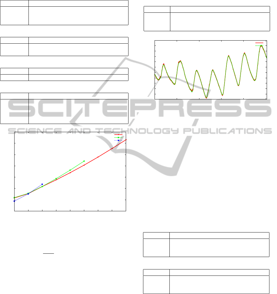
Table 2: Validation partition NRMSE/MAE on mean tem-

perature computed over different future windows.

First hour

Model 0–20 0–40 0–60

NN–060 0.011/0.018 0.019/0.030 0.030/0.047

NN–120 0.014/0.024 0.020/0.031 0.028/0.043

NN–180 0.021/0.034 0.024/0.038 0.029/0.045

Second hour

Model 60–80 60–100 60–120

NN–120 0.067/0.103 0.077/0.120 0.088/0.137

NN–180 0.060/0.094 0.069/0.108 0.079/0.122

Third hour

Model 120–140 120–160 120–180

NN–180 0.121/0.188 0.132/0.205 0.144/0.223

Full interval

Model 0–60 0–120 0–180

NN–060 0.030/0.047 – –

NN–120 0.028/0.043 0.057/0.088 –

NN–180 0.029/0.045 0.052/0.081 0.082/0.126

NN–MIX 0.027/0.043 0.052/0.081 0.082/0.126

0.00

0.02

0.04

0.06

0.08

0.10

0.12

0.14

20 40 60 80 100 120 140 160 180

MAE

Window upper bound

NN−060

NN−120

NN−MIX

Figure 4: Plot of the MAE error computed over the mean of

forecasting windows 0–20, 0–40, 0–60, 0–80, . . . , 0–180,

using NN–060, NN–120, and NN–MIX models.

(

for 0 ≤ i < 60

for 60 ≤ i < 180

(5)

being o

the i-th output of the NN–060 (small model),

and o

the i-th output of the NN–180 (large model).

The combination results are shown on Table 2 and

Figure 4. As we could predict, the NN–MIX model

has a behavior comparable to NN–060 on windows of

size less than 60, and the same behavior as NN–180

for bigger windows.

5.3 Final Results

In order to do a further evaluation of the NN–MIX

model, we compute the NRMSE and MAE measures

for the mean, maximum, and minimum temperatures

Table 3: NRMSE/MAE on minimum, maximum, and mean

temperature forecasting on validation dataset and window

intervals for one, two, and three hours ahead, using the NN–

MIX model.

Window Min Max Mean

0–60 0.029/0.050 0.047/0.061 0.027/0.043

60–120 0.068/0.115 0.099/0.135 0.079/0.122

120–180 0.129/0.214 0.165/0.233 0.143/0.223

0 2000 4000 6000 8000 10000

ºC

Time (minutes)

NN−MIX

Ground Truth

Figure 5: Plot of the forecasted mean temperature versus

ground truth mean temperature using a forecasting window

of 0–60 and the NN–MIX model on the validation partition.

of each forecasting window. The results are shown

on Table 3, showing that mean and minimum temper-

ature measures achieve similar errors, and maximum

temperatures are little worst. We do the same exper-

iment using the unseen test partition. Figure 5 plots

the mean temperature forecasted for the window 0–

60 compared with the ground truth mean temperature

on validation partition.

Table 4: NRMSE/MAE on minimum, maximum, and mean

errors on test dataset and window intervals for one, two, and

three hours ahead, using the NN–MIX model. For compar-

ison purposes NN–ITE model results are shown.

NN–MIX model results

Window Min Max Mean

0–60 0.139/0.188 0.173/0.254 0.150/0.205

60–120 0.255/0.371 0.239/0.360 0.270/0.394

120–180 0.334/0.539 0.381/0.603 0.352/0.566

NN–ITE model results

Window Min Max Mean

0–60 0.402/0.605 0.164/0.257 0.275/0.441

60–120 0.605/0.996 0.519/0.888 0.567/0.956

120–180 0.727/1.249 0.717/1.260 0.723/1.260

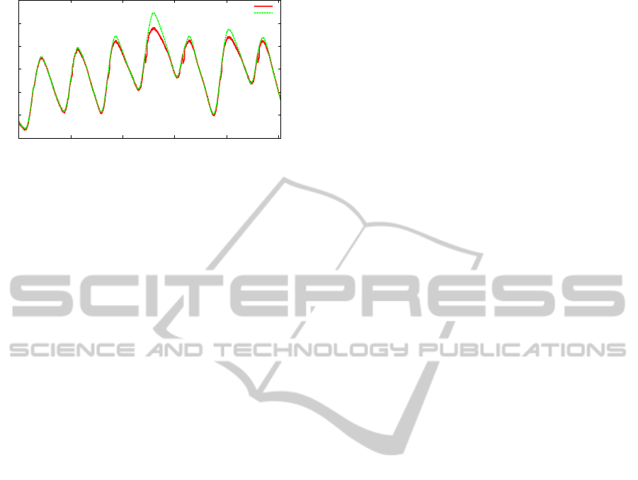
The test partition results are shown on Table 4.

Test partition temperatures are bigger than training

partition temperatures. This leads to bigger errors

on forecasted values. Figure 6 plots the mean tem-

perature forecasted for the window 0–60 compared

with the ground truth mean temperature on test par-

tition. The addition of more training data from differ-

ent months will improve the errors of the model due

to the differences of temperatures between months.

KDIR2012-InternationalConferenceonKnowledgeDiscoveryandInformationRetrieval

210

0 2000 4000 6000 8000 10000

ºC

Time (minutes)

NN−MIX

Ground Truth

Figure 6: Plot of the forecasted mean temperature versus

ground truth mean temperature using a forecasting window

of 0–60 and the NN–MIX model on the test partition.

For comparison purposes we trained an ANN to

predict only the next future value, building iteratively

a window of 180 minutes forecasted values (iterative

multi-step-ahead forecasting). Table 4 shows their re-

sults denoted by NN–ITE. We observe that our ap-

proach outperforms NN–ITE because ANNs trained

using a future window of size greater than one, could

update all their weights using the whole output pre-

diction, and better results are expected (Zhang et al.,

1998).

6 CONCLUSIONS AND FUTURE

WORK

The present paper has shown, in a slightly manner,

the architecture of both hardware and software CAES

system. This has been developed for the SMLhouse

project at our University, which will compete in in-

ternational events. The system is already running and

preliminary data for system validation has been ob-

tained. At the ﬁrst stage, it has been developed all the

monitoring and control architecture, ensuring overall

system reliability. Regarding the intelligent control of

the house, a preliminary version of a rule-based sys-

tem has been developed .

An ANN for indoor temperature prediction has

been implemented, which seems very promising, but

it has to be applied to the rest of the subsystems. Er-

ror achieved by ANNs is little enough to be accepted

by a human being, i.e. it is not perceptible by a per-

son. The proposed ANN model achieve its goals; it is

possible to obtain predictions about maximum, min-

imum and average temperature up to 3 hours with a

MAE close to 0.6

◦

C, and a prediction from one to two

hours with a MAE less than 0.5

◦

C. Such error degree

allows us to think about the possibility of developing

a more complex intelligent module as stated before. It

will be necessary to include other parameters such as

solar intensity, external temperature, humidity, CO

etc. as inputs of the neural network to improve the

predictions. Another idea is to calculate the level of

conﬁdence in the prediction, based on works as (Car-

ney et al., 1999). Other interesting future work will

be to replace current feed-forward ANN with a Long-

Short Term Memory (LSTM) (Graves et al., 2009)

which are a kind of recurrent neural network that is

obtaining impressive results on automatic process and

labeling of sequences due to their superior ability to

model long term dependencies.

ACKNOWLEDGEMENTS

This work was partially supported by IDIT-Santander.

REFERENCES

Bishop, C. M. (1995). Neural networks for pattern recog-

nition. Oxford University Press.

Carney, J., Cunningham, P., Bhagwan, U., and England, L.

(1999). Conﬁdence and Prediction Intervals for Neu-

ral Network Ensembles. In IEEE IJCNN, pages 1215–

1218.

Cheng, H., Tan, P.-n., Gao, J., and Scripps, J. (2006).

Multistep-ahead time series prediction. LNCS,

3918:765–774.

Graves, A. et al. (2009). A Novel Connectionist System

for Unconstrained Handwriting Recognition. IEEE

TPAMI, 31(5):855–868.

Instituto para la diversiﬁcaci

on y ahorro de la energ

ıa

(IDAE) (2011). Practical Guide to Energy. Efﬁcient

and Responsible Consumption. Madrid.

Kreuzer, K. and Eichst

adt-Engelen, T. (2011). The

OSGI-based Open Home Automation Bus.

http://www.openhab.org.

Thomas, B. and Soleimani-Mohseni, M. (2006). Artiﬁcial

neural network models for indoor temperature predic-

tion: investigations in two buildings. Neural Comput.

Appl., 16(1):81–89.

Yu, L., Wang, S., and Lai, K. K. (2008). Forecasting crude

oil price with an EMD-based neural network ensemble

learning paradigm. Energy Economics, 30(5):2623–

2635.

Zhang, G., Patuwo, B. E., and Hu, M. Y. (1998). Forecast-

ing with artiﬁcial neural networks: The state of the art.

International Journal of Forecasting, 14(1):35–62.

SomeEmpiricalEvaluationsofaTemperatureForecastingModulebasedonArtificialNeuralNetworksforaDomotic

HomeEnvironment

211