
GPU-based Parallel Implementation of a Growing
Self-organizing Network
Giacomo Parigi
1∗
, Angelo Stramieri
1
, Danilo Pau
2
and Marco Piastra
1
1
Computer Vision and Multimedia Lab, University of Pavia, Via Ferrata 1 27100, Pavia, PV, Italy
2
Advanced System Technology, STMicroelectronics, Via Olivetti 2 20864, Agrate Brianza, MB, Italy
Keywords:
Growing Self-organizing Networks, Graphics Processing Unit, Parallelism, Surface Reconstruction, Topology
Preservation.
Abstract:
Self-organizing systems are characterized by an inherently local behavior, as their configuration is almost
exclusively determined by the union of the states of each of the units composing the system. Moreover, all
state changes are mutually independent and governed by the same laws. In this work we study the parallel
implementation of a specific subset of this broader family, namely that of growing self-organizing networks,
in relation to parallel computing hardware devices based on Graphic Processing Units (GPUs), which are
increasingly gaining popularity due to their favourable cost/performance ratio. In order to do so, we first
define a new version of the standard, sequential algorithm, where the intrinsic parallelism of the execution is
made more explicit and then we perform comparative experiments with the standard algorithm, together with
an optimized variant of the latter, where an hash index is used for speed. Our experiments demonstrates that
the parallel version outperforms both variants of the sequential algorithm but also reveals a few interesting
differences in the overall behavior of the system, that might be relevant for further investigations.
1 INTRODUCTION
Self-organizing systems are characterized by an in-
herently local behavior, as their configuration at any
instant of the learning process is almost entirely
defined by the union of the states of each of the
units composing the system. The final configuration
reached by such systems, in the case of a successful
execution, will match a set of application-specific cri-
teria, determined by the goal of the system and pos-
sibly by other constraints imposed by the application
field. Generally speaking, the elements composing a
self-organizing system are units executing the same
set of instructions, that are linked together by a set of
connections determining the network topology. The
behavior of each unit is ruled by local informations
only, like the distance from an input signal or the state
of neighboring units. Units in a self-organizing net-
work are usually considered to be totally connected to
the so called input layer, in the sense that each input
signal presented to the network has to be compared to
each and every unit in the network, in order to choose
which is the fittest for this particular input, according
to some metrics, which is called winner unit. Then the
winner unit, together with some form of neighborho-
∗
Corresponding author: giacomo.parigi@gmail.com
od in the network, is adapted to match the input sig-
nal. As a matter of fact, the vast majority of the al-
gorithms of this kind do not make use of any global
variable, besides the complex of units in the network.
This structure seems ideal for a parallel realiza-
tion, despite that the best-known algorithms for self-
organizing systems, like Kohonen’s Self-organizing
Map (SOM) (Kohonen, 1990), Neural Gas (NG)
(Martinetz and Schulten, 1994), Growing Neural Gas
(GNG) (Fritzke, 1995) and Grow-When-Required
networks (GWR) (Marsland et al., 2002) are inher-
ently sequential. The parallelization of growing self-
organizing networks, like GNG and GWR, can be
even more challenging in general given they can grow
or shrink the number of units and/or the topology of
connections during the learning process. On the other
hand, growing self-organizing networks offer some
advantages in that they can often represent the in-
put pattern more accurately and more parsimoniously
(Fritzke, 1995).
In these last years, Graphics Processing Units
(GPU) have rapidly evolved from being purpose-
specific hardware devices into general-purpose paral-
lel computing tools, having also gained a large popu-
larity due to the much lower costs compared to those
of more traditional high-performance computing so-
lutions. In addition, GPU’s rapid increase in both
633
Parigi G., Stramieri A., Pau D. and Piastra M..
GPU-based Parallel Implementation of a Growing Self-organizing Network.
DOI: 10.5220/0004133806330643
In Proceedings of the 9th International Conference on Informatics in Control, Automation and Robotics (ANNIIP-2012), pages 633-643
ISBN: 978-989-8565-21-1
Copyright
c
2012 SCITEPRESS (Science and Technology Publications, Lda.)
programmability and capability has made GPU-based
parallelization the first choice for many applications.
The typical approach to GPU-based paralleliza-
tion for growing self-organizing systems is to adapt a
sequential algorithm, although this might entail some
limitations, as explained in section 2. In this paper we
define a new version of the algorithm for a specific,
growing self-organizing system in which several input
signals are processed simultaneously in each iteration,
instead of just one. The resulting iteration complexity
is higher than the one in the original sequential algo-
rithm, as described in section 3.2, but the net gain is
a substantial speed-up of the whole execution and a
much better tunability of the level of parallelism.
The remainder of the paper is organized as fol-
lows: after a brief description of related works, sec-
tion 3.1 provides a detailed description of features
and limitations of the GPU-based parallel execution
model and section 3.2 describes the learning pro-
cess of growing self-organizing networks. Section 3.3
presents the new algorithm proposed in this paper and
its GPU-based implementation, while section 3.4 de-
scribes an optimized implementation of the sequen-
tial algorithm used for comparison. Finally in section
4 we describe some experiments of this parallel algo-
rithm implemented both for GPU-based and for CPU
execution, compared with the results of the basic se-
quential algorithm and of the opitmized one, followed
by our major conclusions.
2 RELATED WORKS
As it will be explained in section 3.2, the most time-
consuming part of these algorithms is the search for
the winner unit, and therefore most of the optimiza-
tion efforts described in the literature focus on this
aspect. One of the most common approaches, de-
scribed in (Garc
´
ıa-Rodr
´
ıguez et al., 2011) for the
GNG algorithm and in (Campbell et al., 2005) for
the Parameter-Less SOM (PLSOM), is dividing this
search into two different procedures, to be executed
one after the other. The first procedure computes
the distances of each unit from the input signal, and
the second one searches the minimum value, or val-
ues, between those distances. Both of them allow
a straightforward GPU-based parallelization: all the
distances are calculated on the GPU in parallel and
then the minimum is found with a method called par-
allel reduction (Harris, 2007). This approach, how-
ever, needs a direct correspondence between net units
and GPU threads, therefore limiting the maximum
level of parallelism to the number of units currently
in the network. Since growing networks usually start
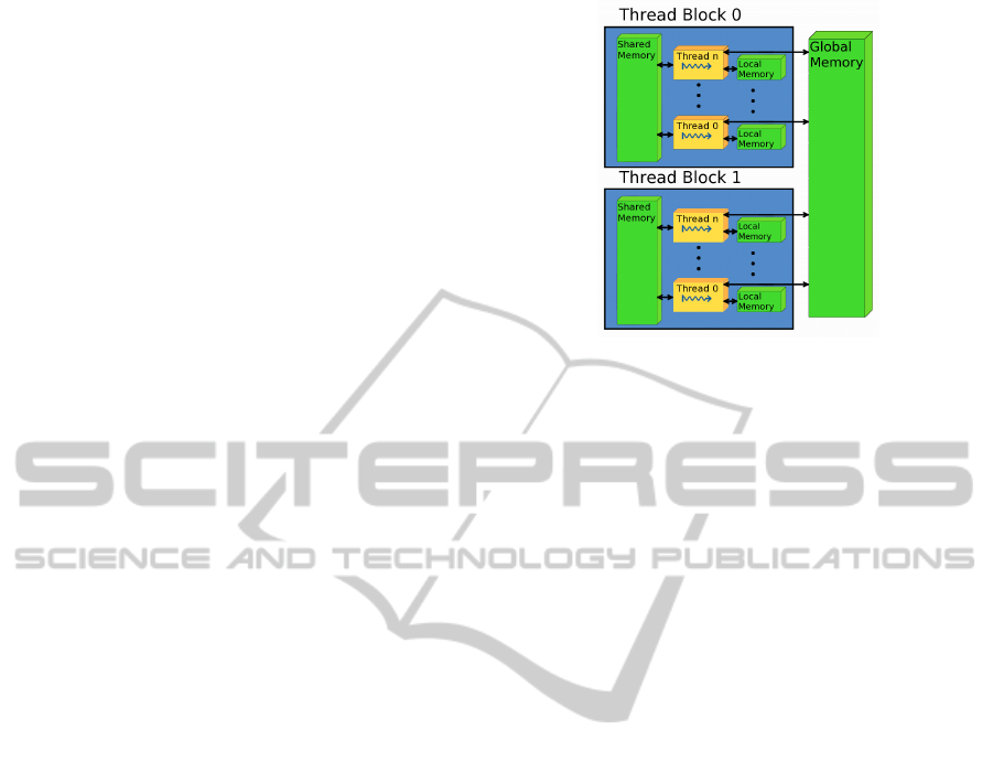
Figure 1: Standard GPU memory hierarchy.
with a very small number of units, this limitation has a
substantial drawback and, in fact, until the net reaches
a size of 500-1000 units, the sequential execution on
a CPU can be faster than the parallel one. A poten-
tial solution, as described in (Garc
´
ıa-Rodr
´
ıguez et al.,
2011), is to apply hybrid techniques, switching the
execution from CPU to GPU only when the latter is
expected to perform better.
The described approach follows a pattern called
map-reduce, which is often used in parallel program-
ming and has been studied and optimized in general
(Liu et al., 2011) and applied to the search of k near-
est neighbors (k-NN) (Zhang et al., 2012). Nonethe-
less, the limit over the level of parallelism imposed
by this method in the case of self-organizing networks
induced the authors to look for alternative paradigms,
as explained in section 3.3, more similar to the paral-
lel brute-force k-NN described in (Garcia et al., 2008)
than to the map-reduce model.
3 METHODS
3.1 Graphics Processing Units
GPUs are specialized processing units optimized for
graphic applications, typically mounted on dedicated
boards with private onboard memory. In these last
years, GPUs have evolved into general-purpose par-
allel execution machines (Owens et al., 2008). Not
all computing tasks are suitable, however, for GPU-
based parallelism. The two relevant aspects for suit-
ability are:
• the level of intrinsic parallelism of the computing
task must be high, in the order of thousands of
threads and more;
• the computing task must be suitable for a SIMD
(Single-Instruction Multiple-Data), at least in the
ICINCO2012-9thInternationalConferenceonInformaticsinControl,AutomationandRobotics
634
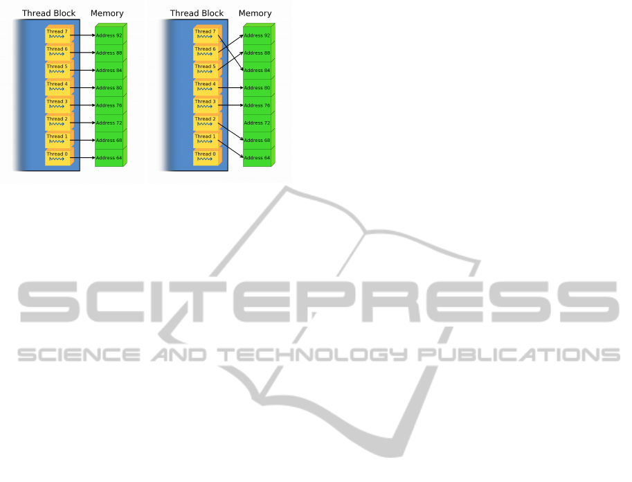
Figure 2: A coherent memory access from a block of
threads, compared to an incoherent one.
variant that is typical to GPU (see below).
Until not many years ago, the only available pro-
gramming interfaces (API) for GPUs were very spe-
cific, forcing the programmer to translate the task into
the graphic primitives provided. Gradually, many
general-purpose API for parallel computing, includ-
ing GPUs, have emerged, like RapidMind (McCool,
2006), PeakStream (Papakipos, 2007) or the program-
ming systems owned by NVIDIA and AMD, respec-
tively CUDA (Compute Unified Device Architecture)
(Nvidia, 2011) and CTM (Close to Metal) (Hensley,
2007), together with proposed vendor-independent
standards like OpenCL (Stone et al., 2010).
Albeit with many non-negligible differences, all
these APIs adopt the general model of stream com-
puting: each element in a set of streams, i.e. ordered
sets of data, is processed by the same kernel, i.e. the
set of functions, to produce one or more streams as
output (Buck et al., 2004).
Each kernel is distributed on a set of GPU cores
in the form of threads, each one executing concur-
rently the same program on a different set of data.
Within this, threads are grouped into blocks and ex-
ecuted in sync: in case of a branching in the exe-
cution the block is partitioned in two, then all the
threads on the first branch are executed in parallel
and eventually the same is done for all the threads
on the second branch. This general model of paral-
lel execution is often called SIMT (single-instruction
multiple-thread) or SPMD (single-program multiple-
data); compared to the older SIMD, it allows greater
flexibility in the flow of different threads, although at
the cost of a certain degree of serialization, depending
on the program. This means that, although indepen-
dent thread executions are possible, blocks of coher-
ent threads with limited branching will make better
use of the GPU’s hardware.
Another noteworthy feature of modern GPUs is
the wide-bandwidth access to onboard memory, on
the order of 10x the memory access bandwidth on
typical PC platforms. To achieve best performances,
however, memory accesses by individual threads
should be made coherent, in order to coalesce them
into fewer, parallel accesses addressing larger blocks
of memory. Figure 2 shows a simple coalesced mem-
ory access compared to an incoherent one. Incoher-
ent accesses, on the other hand, must be divided into
a larger number of sequential memory operations.
In typical GPU architectures, onboard memory
(also called device memory) is organized in a hierar-
chy (Fig.1): global memory, accessible by all threads
in execution, shared memory, a faster cache memory
dedicated to each single thread block and local mem-
ory and/or registers, which are private to each thread.
One of the aspects that make GPU programming
still quite complex, at least with most general purpose
GPU languages, is that the three above levels, in par-
ticular the intermediate cache, have to be managed ex-
plicitly by the programmer. In return, this typically
allows achieving better performances.
3.2 Growing Self-organizing Networks
We consider here self-organizing networks of con-
nected units like GNG (Fritzke, 1995), GWR (Mars-
land et al., 2002) and SOAM (Piastra, 2009) that share
the following characteristics:
• the number of units varies, typically growing dur-
ing the learning process;
• the topology of connections between units varies
as well, and connections are both created and de-
stroyed during the learning process.
Moreover, like with most self-organizing networks,
each unit is associated to a reference vector in the in-
put space, which is progressively adapted during the
learning process.
In general, in the learning process of a growing
self-organizing network, a basic iteration step is re-
peated until some convergence criterion is met. The
typical iteration can be described as follows:
1. Sample
Generate at random one input signal ξ with prob-
ability P(ξ).
2. Find Winners
Compute the distances kξ−w
i
k between each ref-
erence vector and the input signal and find the k-
nearest units. In most cases, k = 2: the winner
(nearest) and second-nearest units are searched
for.
3. Update the Network
Create a new connection between the winner and
the second-nearest unit, if not existing, or reset the
GPU-basedParallelImplementationofaGrowingSelf-organizingNetwork
635
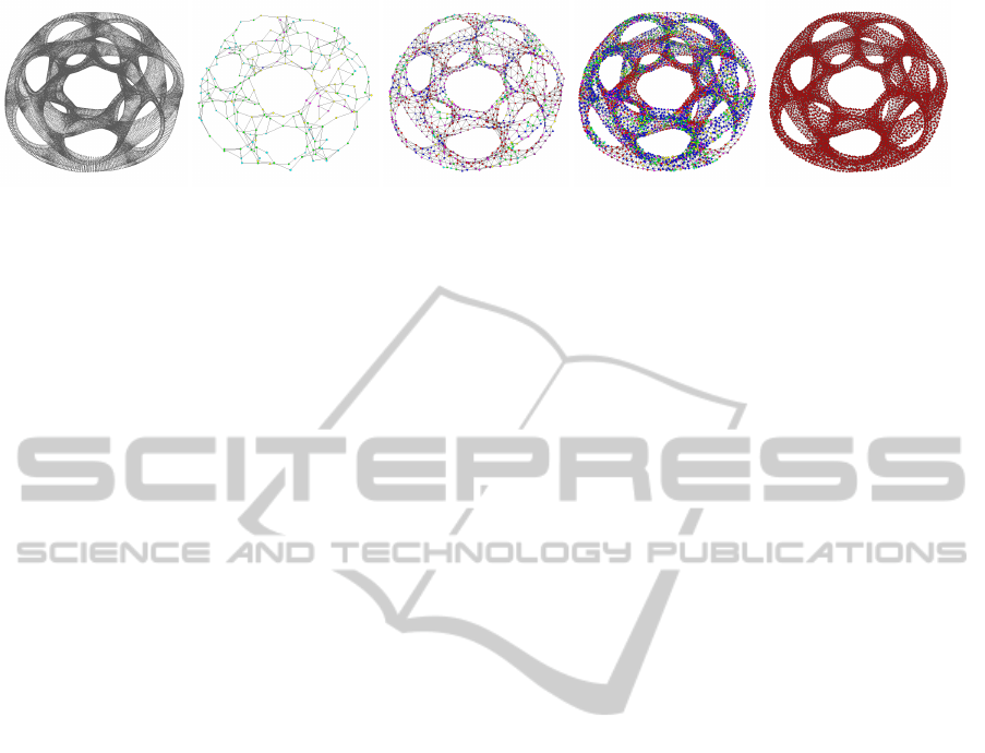
Figure 3: The SOAM (Piastra, 2009) reconstructs a surface from the point cloud on left. At the end, all units converge to the
same stable state.
existing one. An aging mechanism is also applied
to connections (see for instance (Fritzke, 1995)).
Adapt the reference vector of the best matching
unit and of its topological neighbors, in most cases
with the law:
∆w
b
= ε
b
kξ − w
b
k,
∆w
i
= ε
i
η(i, b)kξ − w
i
k,
where w
b
is the reference vector of the winner and
w
i
are the reference vectors of all other units in
the network. ε
b
, ε
i
, ∈ [0, 1] are learning rates, with
ε
b
ε
i
. The function η(i, b) ≤ 1 determines how
other units are adapted. In many cases η(i, b) = 1
if units b and i are connected and 0 otherwise.
During the Update phase, new units are both cre-
ated and removed, with methods that may vary de-
pending on the specific algorithm (see below).
In the discussion that follows we will not consider
the Sample phase in detail. Sampling methods, in fact,
are application-dependent and not necessarily under
the control of the algorithm.
Clearly, assuming that k is constant and small
w.r.t. the number of units N, the Find Winners phase
has O(N) time complexity. The complexity of the Up-
date phase depends in general from how the function
η(i, b) is defined. For instance, with the Neural Gas
algorithm (Martinetz and Schulten, 1994), this step
is dominant, as it involves all units in the network
and requires an O(N log N) time. In this discussion
we will content ourselves with the very frequent case
where the update is limited to the connected neigh-
bors of the winner. This means that, under these con-
ditions, the Update phase can be assumed to have
O(1) time complexity.
The Find Winners phase hence dominates the
complexity of the execution and must be the main fo-
cus for optimization and/or parallelization. The graph
in Fig.6 shows the experimental results that confirm
the assumptions above for two of the meshes used in
the experimental phase, described in Section 4.
Growing self-organizing networks are capable of
adding units to the network following algorithm-
specific patterns, during the Update phase. In GNG,
new units are inserted at regular intervals, in the
neighborhood of the unit i that has accumulated the
largest average error kξ − w
i
k as winner. In contrast,
in GWR new units are added whenever the input sig-
nal ξ is farther away than a predefined threshold from
the winner unit.
In SOAM the latter threshold may vary during the
learning process depending on the topology of the
neighborhood of units. In addition, the SOAM al-
gorithm introduces a clear termination criterion that
does not depend on a parameter and is met when all
the units have an expected neighborhood topology,
thus allowing a better comparison of performances.
3.3 Parallel Implementation
In the sequential iteration described in the previous
section, the maximum possible parallelism for the
dominant Find Winners phase can be obtained by
computing all the distances between all the reference
vectors w
i
and the (unique) signal ξ in parallel and
then reducing the set to the k closest reference vec-
tors. This method has an intrinsic limit in the maxi-
mum level of parallelism, which is bound to the cur-
rent number of units in the network, that becomes
even more relevant when reducing to the k closest ref-
erence vectors.
In order to better harness the parallel execution
model, we prefer adopting a different algorithm where
at each iteration m 1 signals are considered at once.
In this variant, the basic iteration step can be de-
scribed as follows:
1. Sample
Generate at random m input signals ξ
1
, . . . , ξ
m
ac-
cording to the probability distribution P(ξ).
2. Find Winners
In parallel, for each signal ξ
j
, compute the dis-
tances kξ
j
− w
i
k between each reference vector
and the input signal and find the k-nearest units.
3. Update the Network
Perform the update operations as specified in the
previous section, but for each signal ξ
j
.
The kernel that is executed for the above search
in the Find Winners phase, comprises two step (see
ICINCO2012-9thInternationalConferenceonInformaticsinControl,AutomationandRobotics
636
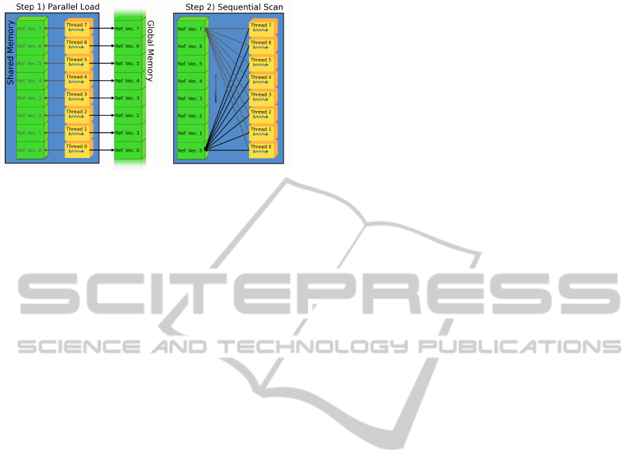
Figure 4: The two steps of the Find Winners phase in the
presented algorithm.
Fig.4): first, all threads in a block load a contiguous
batch of reference vectors in the shared memory with
a coalesced access; second, all threads perform a se-
quential scan of the shared memory where at each
pass they all read same reference vector and com-
pute the corresponding distance in parallel. From the
point of view of GPU-based parallelization, the latter
schema has several advantage, most of all permitting
a simple and effective management of the faster and
smaller shared memory in order to accelerate the ac-
cess to the global memory, which is the only that can
store all the reference vectors at once.
A GPU implementation that follows this approach
could maintain, in theory, the same level of paral-
lelism m across the entire execution of the kernel, as
no reduction takes place. Furthermore, still in the-
ory, there is no upper limit for the level of parallelism
m beyond that of the hardware. However, in order
to make this possibility actual, the collisions occur-
ring when two or more samples share the same winner
units must be managed in the Update phase.
In the actual implementation presented here, we
adopted a simplified sequential method for managing
collisions in the Update phase, in that we avoid collid-
ing adaptations of the same reference vector by adapt-
ing any unit to the first signal for which it is winner, in
the ordering of threads, and just discarding any other
signals for which that same unit is winner in the same
iteration.
For this study we used the SOAM algorithm, al-
though we expect the results obtained to be valid for a
larger class of growing self-organizing networks, for
the reasons described in section 3.2.
To better test this approach an intermediate pro-
gram version has been realized, simulating parallel
behavior inside a sequential program, i.e. performing
parallel sections of the code as ‘for’ cycles.
3.4 Hash Indexing
As known, there is no a priori warranty that a parallel
algorithm should be faster than a highly-optimized se-
quential one. Therefore we chose to compare the par-
allel algorithm not only to its basic sequential coun-
terpart but also to a variant in which the crucial Find
Winners phase is improved through the use of a hash
indexing method, similar to that used in molecular dy-
namics simulations (Hockney and Eastwood, 1988).
This hash index is constructed by first identifying
an axis-parallel bounding box in the input space that
contains all the input signals. The bounding box is
then divided in a grid of cubes of fixed side, and for
each cube an hash index is obtained from the coordi-
nates of its major corner. Every reference vector con-
tained in the same cube, called index box, is bound
to have the same hash index, and it will be retrieved
from that, during the Find Winners phase.
During Update phase, the reference vectors of the
winner and its neighboring units are adapted and this
entails updating the index as well. The hash index
adopted here is particularly efficient with the inser-
tion, update and removal of reference vectors but it
also introduces some sort of approximation, as it in-
volves approximating a sphere (i.e. around the signal)
with a cube. Experiments show that the differences in
the overall behavior due to this approximate search
strategy are negligible.
4 EXPERIMENTAL RESULTS
All the experiments described in this section have
been performed with the SOAM algorithm, in four
different implementations (see below), applied to the
task of surface reconstruction from point clouds. In
each experiment, a triangular mesh was considered as
the source for the point cloud; the vertices of the mesh
were selected as input signals in the Sample phase
with uniform probability distribution P(ξ).
Four different meshes have been used for the com-
parative benchmark, each having different topologi-
cal and geometrical complexity. More precisely, we
consider two measures, corresponding to each type of
complexity: the genus of the surface (Edelsbrunner,
2006), i.e. the number of holes through it, and the lo-
cal feature size (LFS), that is defined in each point x
as the Euclidean distance from x to (the nearest point
of) the medial axis (Amenta and Bern, 1999). In this
perspective, a mesh is deemed here “simple” if it has
either genus zero or very low and is characterized by
a high and relatively constant LFS, while it is deemed
“complex” if it has higher genus and LFS values that
GPU-basedParallelImplementationofaGrowingSelf-organizingNetwork
637
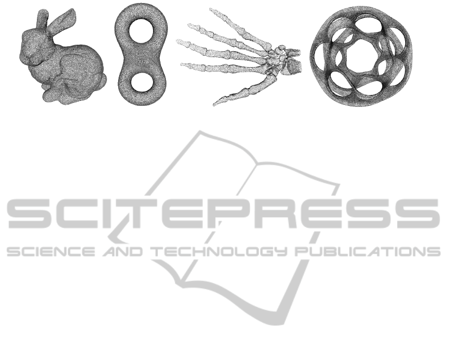
Figure 5: The four point-clouds used in the test phase.
vary widely across different areas.
The meshes used in the experiments, coming from
well-known benchmarks for surface reconstruction,
are the following (Fig. 5):
• Stanford Bunny. Is the “simplest” mesh used, with
genus 0 although with some non-negligible varia-
tions in the LFS that make it non-trivial.
• Eight (also called double torus). it has genus 2
and a relatively constant LFS almost everywhere.
It is deemed “simple” for the purposes of our dis-
cussion.
• Hand. It represents the skeleton of a hand. It has
genus 5 and a highly variable LFS, that in many
areas, e.g. close to the wrist, becomes consider-
ably low. It is a “complex” mesh.
• Heptoroid. Is the most “complex” mesh used,
having genus 22, and a variable and generally low
LFS for the most part of it.
Four different implementation of the basic SOAM
algorithms have been used for the experiments:
• Sequential. A reference implementation of the ba-
sic, sequential SOAM algorithm in C.
• Indexed. The same sequential algorithm as above
but using an hash index for the Find Winners
phase.
• Simulated Parallel. A reference implementation
in C of the new version proposed for the algo-
rithm, as described in Section 3.3 but without any
actual parallelization, in terms of execution.
• GPU-based. An implementation in C and
NVIDIA C/CUDA of the new version proposed
for the algorithm, with true hardware paralleliza-
tion.
The tests have been performed on a Dell Preci-
sion T3400 workstation, with a NVidia GeForce GT
440, i.e. an entry-level GPU based on the Fermi archi-
tecture. The operating system is MS Windows Vista
Business SP2 and all the programs have been com-
piled with MS Visual C++ Express 2010, with the
CUDA SDK version 4.0.
All the parameters shared across the four different
implementations have been set to the same values for
all the tests, while algorithm-specific parameters, as
parallelism level or index box side, have been tuned to
obtain maximum performances. Only one fundamen-
tal parameter, the insertion threshold has been tuned
for each mesh, although the value of this parameter
depends only on the complexity of the mesh, in the
above sense (see also (Piastra, 2009)), and not on the
specific implementation of the algorithm.
In order to avoid discarding an excessive number
of signals in the Update phase, in all parallel imple-
mentations the level of parallelism m at each iteration
is set to the minimum power of two greater than the
current number of units in the network. The maxi-
mum level of parallelism has been set to 8192.
The numerical results obtained from the experi-
ments are given in tables 1, 2, 3, and 4, at the end of
this section. As it can be seen, for each input mesh,
the different implementations reach final configura-
tions with very different number of units and connec-
tions, also requiring a different number of signals for
convergence. Simulated parallel and GPU-based im-
plementations, in contrast, produce exactly the same
numbers since they are meant to replicate the same
behavior, for validation.
As expected, substantial differences are also vis-
ible for the execution times. In the tables, these
times are reported as total times to convergence and
times per signal, together with the details of each of
the three phases. Times per signal are intended as
measures of the raw performances that can be ob-
tained with each implementation, while times to con-
vergence are the combined results of the implementa-
tion and the different behaviors of the two algorithms,
as it will be explained in the next subsections.
4.1 Performances
Fig.6 shows a summary of the times to convergence
for the Sequential, Indexed and GPU-based imple-
mentations respectively, for the two most complex
meshes, divided by phase. Remarkably, in the GPU-
ICINCO2012-9thInternationalConferenceonInformaticsinControl,AutomationandRobotics
638
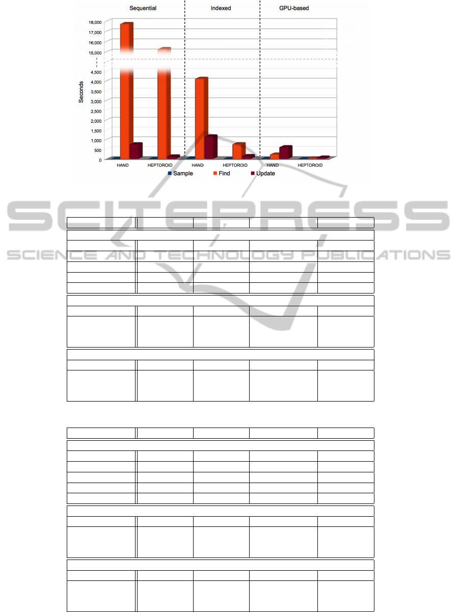
Figure 6: Single-phase time to convergence for the two more complex meshes in the test set.
Table 1: Execution time and statistics on the Stanford Bunny data-set, for the four implementations.
Algorithm Version Sequential Indexed Simulated Parallel GPU-based
Network Configuration at Convergence
Iterations 620,000 616,000 1,296 1,296
Signals 620,000 616,000 580,656 580,656
Discarded Signals 0 0 319,054 319,054
Units 330 332 347 347
Connections 984 990 1,035 1,035
Time to Convergence
Total Time 4.9530 3.369 3.893 2.059
Sample 0.460 0.048 0.009 0.016
Find Winners 2.610 1.233 2.448 0.699
Update 1.883 2.088 1.436 1.344
Times per Signal
Time per Signal 7.9887 × 10
−06
5.4692 × 10
−06
6.7045 × 10
−06
3.5460 × 10
−06
Sample 7.4194 × 10
−07
7.7922 × 10
−08
1.5500 × 10
−08
2.7555 × 10
−08
Find Winners 4.2097 × 10
−06
2.0016 × 10
−06
4.2159 × 10
−06
1.2038 × 10
−06
Update 3.0371 × 10
−06
3.3896 × 10
−06
2.4731 × 10
−06
2.3146 × 10
−06
Table 2: Execution time and statistics on the Eight data-set, for the four implementations.
Algorithm Version Sequential Indexed Simulated Parallel GPU-based
Network Configuration at Convergence
Iterations 1,100,000 1,100,000 1,128 1,128
Signals 1,100,000 1,100,000 1,100,110 1,100,110
Discarded Signals 0 0 562,277 562,277
Units 656 649 658 658
Connections 1,974 1,953 1,980 1,980
Time to Convergence
Total Time 12.3540 5.5690 11.6070 3.8690
Sample 0.0150 0.0480 0.0620 0.1410
Find Winners 8.8600 2.8220 8.5060 0.7650
Update 3.4790 2.6990 3.0390 2.9630
Times per Signal
Time per Signal 1.1231 × 10
−05
5.0627 × 10
−06
1.0551 × 10
−05
3.5169 × 10
−06
Sample 1.3636 × 10
−08
4.3636 × 10
−08
5.6358 × 10
−08
1.2817 × 10
−07
Find Winners 8.0545 × 10
−06
2.5655 × 10
−06
7.7320 × 10
−06
6.9539 × 10
−07
Update 3.1627 × 10
−06
2.4536 × 10
−06
2.7625 × 10
−06
2.6934 × 10
−06
GPU-basedParallelImplementationofaGrowingSelf-organizingNetwork
639
based implementation, the Find Winners phase ceases
to be the dominant one, while the Update phase be-
comes the most time-consuming. This means that in
this implementation further optimizations of the Find
Winners phase are useless unless the execution of the
Update phase is sped up in turn.
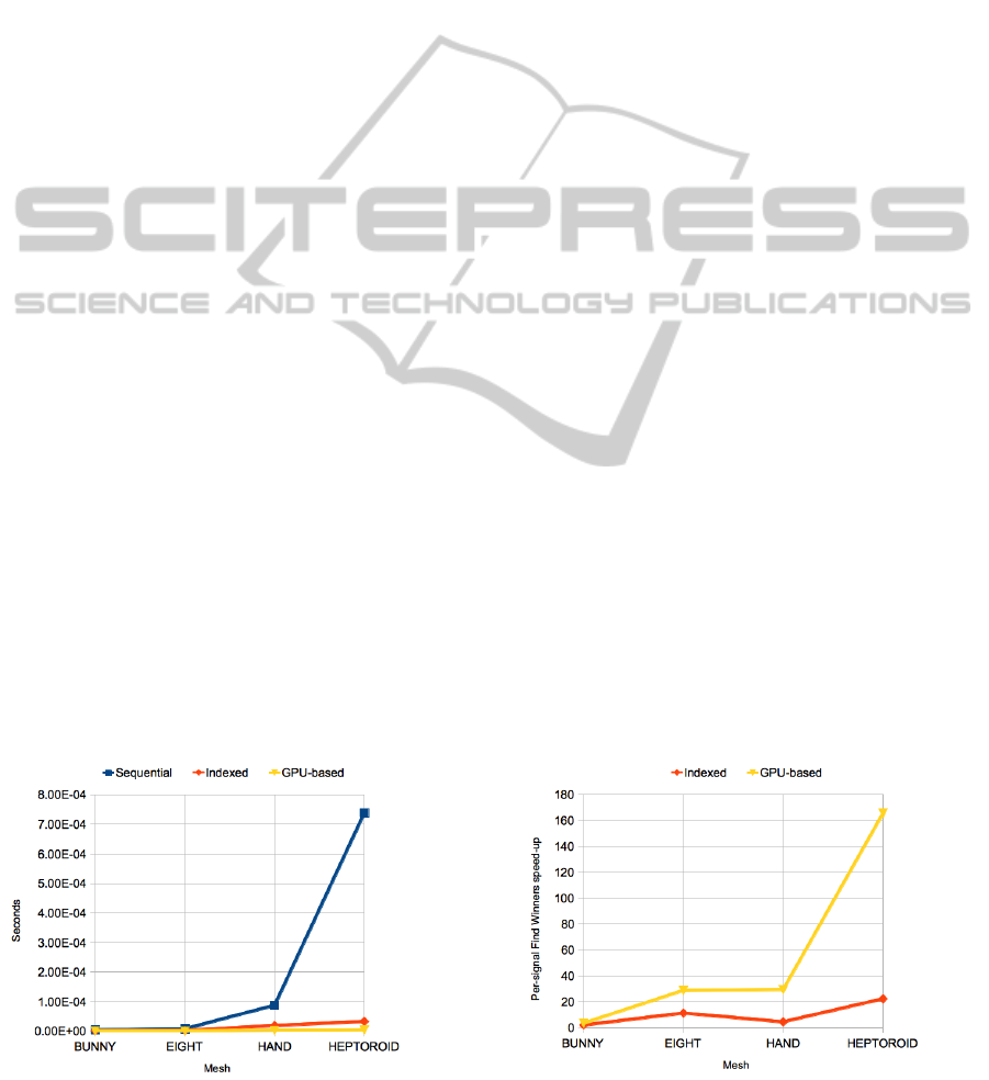
More in detail, Fig.7 shows the average times per
signal spent in the Find Winners phase for the three
implementations. Clearly, these times grow as the
number of the units in the network becomes larger.
Fig.8 shows the speed-up factor, for the same figure,
of the Indexed and GPU-based implementations com-
pared to the Sequential one. As expected, the speed-
up factor also grows with the number of units in the
network, as the hash index in the Indexed implemen-
tation becomes more effective and an higher level of
parallelism can be achieved in the GPU-based imple-
mentation. As it can be seen, the speed-up factor for
the GPU-based implementation reaches 165x on the
Heptoroid mesh.
The total times to convergence are shown in Fig.9.
These results show that the performances of the
SOAM algorithm depend in particular on how much
the LFS varies across the mesh; the hand in fact is
the input mesh that requires the longest time to con-
vergence, regardless of the implementation. Fig.10
shows the speed-up factor for the time to convergence,
once again comparing the Indexed and GPU-based
implementations with the Sequential one; this speed-
up factor too grows with the number of units in the
network.
In every case, the times to convergence for the
GPU-based implementation are much lower than the
ones of the Sequential implementation. Speed-ups
vary from 2.5x (bunny) to 129x (heptoroid), as com-
plexity of the mesh and size of the reconstructed net-
work grow. In particular, the results obtained with the
Stanford Bunny mesh, given in table 1, show non neg-
ligible speed-up factors for both the time to conver-
Figure 7: Times per signal in the Find Winners phase for
the three implementations.
gence (2.5x) and the time per signal in the Find Win-
ners phase (3.5x), despite that network contains only
330-347 units at most. This result is in particular rel-
evant if compared to other GPU-based parallel imple-
mentation of growing self-organizing networks (see
for example (Garc
´
ıa-Rodr
´
ıguez et al., 2011)), where
it is said that GPU-based execution begin to obtain a
noticeable speed-up, with respect to a sequential CPU
execution, with nets of more than 500-1000 units.
The Indexed implementation of the algorithm also
obtains a noticeable speed-up on all the meshes,
namely 1.5x for the Stanford bunny, 2.5x for the
Eight, 3.5x for the Hand and 16x for the heptoroid.
Nonetheless, as shown in Fig.6 in this implementa-
tion the Find Winners phase still remains the domi-
nant one, even if in the simple Stanford bunny and
Eight reconstructions the Update time is comparable.
4.2 Parallel Algorithm Behavior
The results in the first three lines of tables 1, 2, 3 and 4
highlight an aspect that is worth some further discus-
sion. The two algorithms described in Sections 3.2
and 3.3 are different and have in fact different behav-
iors.
The comparison of the number of signals used
by the two implementations shows that the Simulated
parallel implementation always needs a substantially
lower number of input signals than the Sequential im-
plementation to converge. This difference becomes
even more evident if the discarded signals are not
counted for, approaching one to four ratio as the mesh
becomes more complex. This decrease in the number
of signals to convergence is attained in spite of the
growth in the number of units and connections.
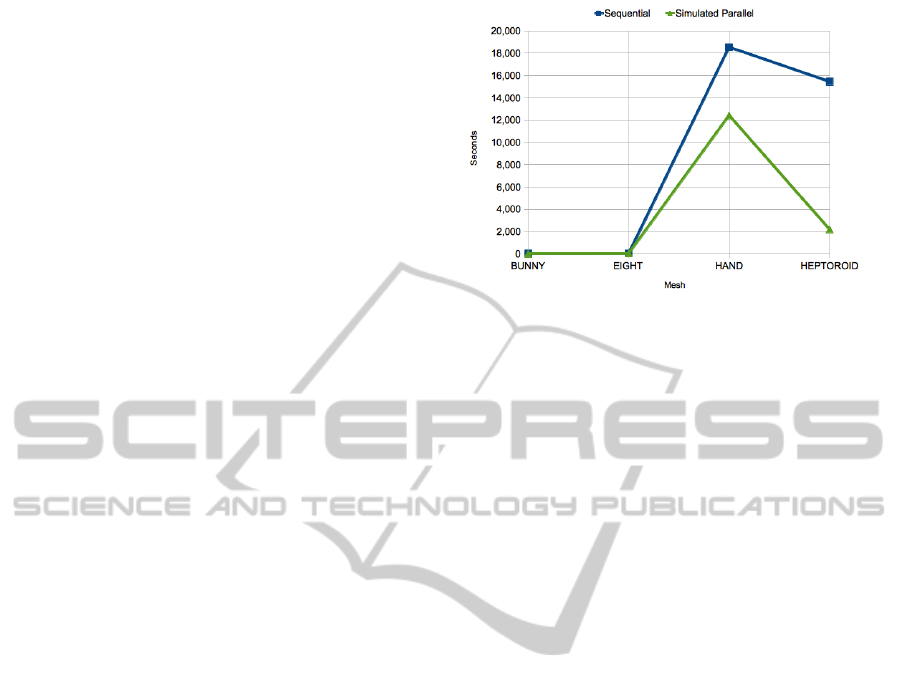
Fig.11 shows the times to convergence of the
Sequential and Simulated parallel implementations.
The performances of Simulated parallel implemen-
tation are always better than its Sequential counter-
Figure 8: Speed-up factors for the Find Winners phase time
per signal compared to the Sequential implementation.
ICINCO2012-9thInternationalConferenceonInformaticsinControl,AutomationandRobotics
640
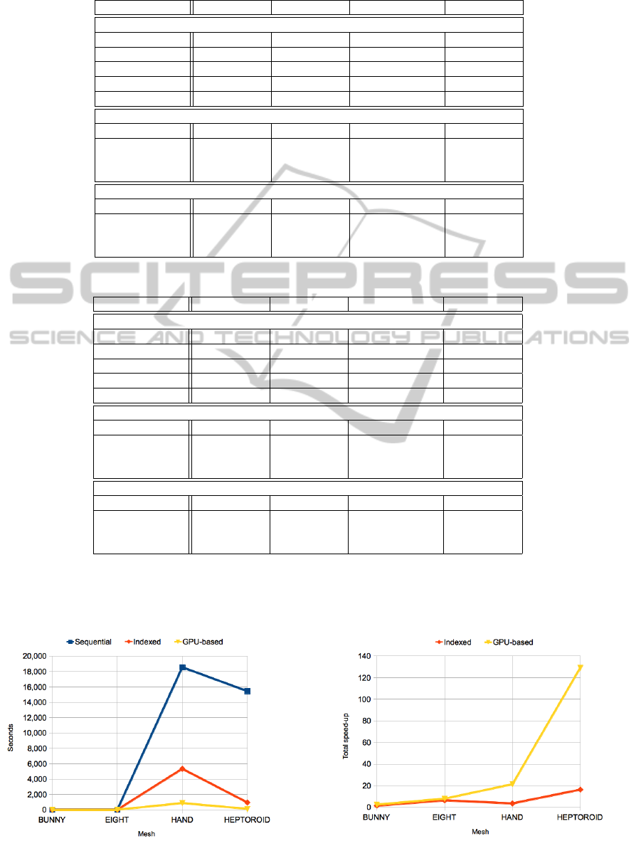
Table 3: Execution time and statistics on the Hand data-set, for the four implementations.
Algorithm Version Sequential Indexed Simulated Parallel GPU-based
Network Configuration at Convergence
Iterations 202,988,000 213,800,000 10.264 10.264
Signals 202,988,000 213,800,000 81.092.912 81.092.912
Discarded Signals 0 0 33.432.622 33.432.622
Units 5,669 5,766 8.884 8.884
Connections 17,037 17,328 26.688 26.688
Time to Convergence
Total Time 18, 548.4937 5, 337.2451 12, 422.3738 872.0250
Sample 9.4050 35.9820 8.6120 8.0480
Find Winners 17, 763.1367 4, 127.8511 11, 789.8398 241.1750
Update 775.9520 1, 173.4120 623.9220 622.8020
Times per Signal
Time per Signal 9.1377 × 10
−05
2.4964 × 10
−05
1.5319 × 10
−04
1.0753 × 10
−05
Sample 4.6333 × 10
−08
1.6830 × 10
−07
1.0620 × 10
−07
9.9244 × 10
−08
Find Winners 8.7508 × 10
−05
1.9307 × 10
−05
1.4539 × 10
−04
2.9741 × 10
−06
Update 3.8226 × 10
−06
5.4884 × 10
−06
7.6939 × 10
−06
7.6801 × 10
−06
Table 4: Execution time and statistics on the Heptoroid data-set, for the four implementations.
Algorithm Version Sequential Indexed Simulated Parallel GPU-based
Network Configuration at Convergence
Iterations 20,714,000 23,684,000 1,244 1,244
Signals 20,714,000 23,684,000 7,683,554 7,683,554
Discarded Signals 0 0 2,262,969 2,262,969
Units 14,183 13,937 15,638 15,638
Connections 42,675 41,937 47,040 47,040
Time to Convergence
Total Time 15, 449.2950 950.0250 2, 172.8009 119.6530
Sample 6.9570 3.4550 0.8010 0.5630
Find Winners 15, 294.3330 780.5370 2, 089.6169 34.2640
Update 148.0050 166.0330 82.3830 84.8260
Times per Signal
Time per Signal 7.4584 × 10
−04
4.0113 × 10
−05
2.8279 × 10
−04
1.5573 × 10
−05
Sample 3.3586 × 10
−07
1.4588 × 10
−07
1.0425 × 10
−07
7.3273 × 10
−08
Find Winners 7.3836 × 10
−04
3.2956 × 10
−05
2.7196 × 10
−04
4.4594 × 10
−06
Update 7.1452 × 10
−06
7.0103 × 10
−06
1.0722 × 10
−05
1.1040 × 10
−05
part, a difference that becomes more substantial as
the complexity of the mesh increases. Overall, this
means that the losses in execution time due to the in-
Figure 9: Times to convergence for the three implementa-
tions.
crease in the number of both units and connections are
outbalanced by the decrease in the number of signals
to converge.
Figure 10: Speed-up factors for the time to convergence
compared to the Sequential implementation.
GPU-basedParallelImplementationofaGrowingSelf-organizingNetwork
641
In a possible explanation, the parallel algorithm
proposed in Section 3.3 has an inherently more dis-
tributed behavior than the original sequential one. In
fact, in each iteration, a number of units scattered ran-
domly along the whole mesh is updated, virtually at
the same time, while in the original algorithm only
the winner unit and its direct neighbors are updated
before the next iteration. This distributed behavior
apparently leads to a more effective use of each input
signal, thus permitting a faster convergence, at least
in terms of input signals needed. This aspect requires
further investigation.
5 CONCLUSIONS AND FUTURE
DEVELOPMENTS
In this paper we examined the GPU-based paralleliza-
tion of a generic, growing self-organizing network by
proposing a parallel version of the original algorithm,
in order to increase its level of scalability.
In particular, the parallel version proposed adapts
more naturally to the GPU architecture, taking advan-
tage of its hierarchical memory access through a care-
ful data placement, of the wide onboard bandwidth
through perfectly coalesced memory accesses, and of
the high number of cores with a scalable level of par-
allelization.
An interesting, and somehow unexpected, aspect
that the experiments have revealed is that - parallel
execution apart - the overall behavior of the parallel
algorithm proposed is different form the original, se-
quential one. The parallel version of the algorithm, in
fact, seems to better deal with complex meshes by re-
quiring a smaller number of signals in order to reach
network convergence. This aspect needs to be inves-
tigated more, with more specific and extensive exper-
iments.
The parallelization described in this paper limited
itself to the Find Winners phase and, according to
the experimental results, succeeds in making it less
time-consuming than the Update phase. This means
that future developments of the algorithm proposed
should aim to the effective parallelization of the Up-
date phase as well, in order to improve on perfor-
mances. This requires some care however, as col-
lisions among threads corresponding to signals for
which the same unit is winner must be treated with
care, even in the light of the limited thread synchro-
nization capabilities implemented on GPUs.
Figure 11: times to convergence of the Sequential and Sim-
ulated parallel implementations.
REFERENCES
Amenta, N. and Bern, M. (1999). Surface reconstruction by
voronoi filtering. Discrete & Computational Geome-
try, 22(4):481–504.
Buck, I., Foley, T., Horn, D., Sugerman, J., Fatahalian, K.,
Houston, M., and Hanrahan, P. (2004). Brook for
gpus: stream computing on graphics hardware. ACM
Transactions on Graphics (TOG), 23(3):777–786.
Campbell, A., Berglund, E., and Streit, A. (2005). Graphics
hardware implementation of the parameter-less self-
organising map. Intelligent Data Engineering and Au-
tomated Learning-IDEAL 2005, pages 5–14.
Edelsbrunner, H. (2006). Geometry and Topology for Mesh
Generation. Cambridge University Press.
Fritzke, B. (1995). A growing neural gas network learns
topologies. In Advances in Neural Information Pro-
cessing Systems 7. MIT Press.
Garcia, V., Debreuve, E., and Barlaud, M. (2008). Fast
k nearest neighbor search using gpu. In Computer
Vision and Pattern Recognition Workshops, 2008.
CVPRW’08. IEEE Computer Society Conference on,
pages 1–6. Ieee.
Garc
´
ıa-Rodr
´
ıguez, J., Angelopoulou, A., Morell, V., Orts,
S., Psarrou, A., and Garc
´
ıa-Chamizo, J. (2011). Fast
image representation with gpu-based growing neural
gas. Advances in Computational Intelligence, pages
58–65.
Harris, M. (2007). Optimizing parallel reduction in cuda.
CUDA SDK Whitepaper.
Hensley, J. (2007). Amd ctm overview. In ACM SIGGRAPH
2007 courses, page 7. ACM.
Hockney, R. W. and Eastwood, J. W. (1988). Computer sim-
ulation using particles. Taylor & Francis, Inc., Bristol,
PA, USA.
Kohonen, T. (1990). The self-organizing map. Proceedings
of the IEEE, 78(9):1464–1480.
Liu, S., Flach, P., and Cristianini, N. (2011). Generic
multiplicative methods for implementing machine
learning algorithms on mapreduce. Arxiv preprint
arXiv:1111.2111.
ICINCO2012-9thInternationalConferenceonInformaticsinControl,AutomationandRobotics
642

Marsland, S., Shapiro, J., and Nehmzow, U. (2002). A self-
organising network that grows when required. Neural
Networks, 15(8-9):1041–1058.
Martinetz, T. and Schulten, K. (1994). Topology represent-
ing networks. Neural Networks, 7(3):507–522.
McCool, M. (2006). Data-parallel programming on the cell
be and the gpu using the rapidmind development plat-
form. In GSPx Multicore Applications Conference,
volume 9.
Nvidia, C. (2011). Nvidia cuda c programming guide.
NVIDIA Corporation.
Owens, J., Houston, M., Luebke, D., Green, S., Stone, J.,
and Phillips, J. (2008). Gpu computing. Proceedings
of the IEEE, 96(5):879–899.
Papakipos, M. (2007). The peakstream platform: High-
productivity software development for multi-core pro-
cessors. PeakStream Inc., Redwood City, CA, USA,
April.
Piastra, M. (2009). A growing self-organizing network for
reconstructing curves and surfaces. In Neural Net-
works, 2009. IJCNN 2009. International Joint Con-
ference on, pages 2533–2540. IEEE.
Stone, J., Gohara, D., and Shi, G. (2010). Opencl: A par-
allel programming standard for heterogeneous com-
puting systems. Computing in science & engineering,
12(3):66.
Zhang, C., Li, F., and Jestes, J. (2012). Efficient parallel knn
joins for large data in mapreduce. In Proceedings of
15th International Conference on Extending Database
Technology (EDBT 2012).
GPU-basedParallelImplementationofaGrowingSelf-organizingNetwork
643
