
A Semi-supervised Learning Framework to Cluster Mixed Data Types
Artur Abdullin and Olfa Nasraoui
Knowledge Discovery & Web Mining Lab, Department of Computer Engineering and Computer Science,
University of Louisville, Louisville, KY, U.S.A.
Keywords:
Semi-supervised Clustering, Mixed Data Type Clustering.
Abstract:
We propose a semi-supervised framework to handle diverse data formats or data with mixed-type attributes.
Our preliminary results in clustering data with mixed numerical and categorical attributes show that the pro-
posed semi-supervised framework gives better clustering results in the categorical domain. Thus the seeds
obtained from clustering the numerical domain give an additional knowledge to the categorical clustering al-
gorithm. Additional results show that our approach has the potential to outperform clustering either domain
on its own or clustering both domains after converting them to the same target domain.
1 INTRODUCTION
Many algorithms exist for clustering. However most
of them have been designed to optimally handle spe-
cific types of data, e.g the spherical k-means was pro-
posed to cluster text data (Dhillon and Modha, 2001).
The algorithm in (Banerjee et al., 2005) has been de-
signed for data with directional distributions that lie
on the unit hypersphere such as text data. The k-
modes has been designed specifically for categorical
data (Huang, 1997). Special data types and domains
have been also handled using specialized dissimilar-
ity or distance measures. For example, the k-means,
using the Euclidean distance, is optimal for compact
globular clusters with numerical attributes.
Suppose that a data set comprises multiple types
of data that can each be best clustered with a different
specialized clustering algorithm or with a specialized
dissimilarity measure. In this case, the most com-
mon approach has been to either convert all data types
to the same type (e.g: from categorical to numerical
or vice-versa) and then cluster the data with a stan-
dard clustering algorithm in that target domain; or to
use a different dissimilarity measure for each domain,
then combine them into one dissimilarity measure and
cluster this dissimilarity matrix with an O(N
2
) algo-
rithm.
To handle possibly diverse data formats and dif-
ferent sources of data, we propose a new approach for
combining diverse representations or types of data.
Examples of data with mixed attributes include net-
work activity data (e.g. the KDD cup data), most
existing census or demographic data, environmental
data, and other scientific data. Our approach is rooted
in Semi-Supervised Learning (SSL), however it uses
SSL in a completely novel way and for a new purpose
that has never been the objective in previous SSL re-
search and applications. More specifically, traditional
semi-supervised learning or transductive learning has
been used mainly to exploit additional information in
unlabeled data to enhance the performance of a clas-
sification model (traditionally trained using only la-
beled data) (Zhu et al., 2003), or to exploit some ex-
ternal supervision in the form of a few labeled data
to improve the results of clustering unlabeled data.
However, in this paper, we will use SSL “without”
any external labels. Rather, the helpful labels will
be “inferred” from multiple Unsupervised Learners
(UL), such that each UL transmits to the other UL,
a subset of confident labels that it has learned on its
own from the data in one domain, along with some of
the data that has been labeled with these newly dis-
covered (cluster) labels. Hence the ULs from the dif-
ferent domains try to guide each other using mutual
semi-supervision.
The rest of this paper is organized as follows. Sec-
tion 2 gives an overview of related work. Section 3
presents our proposed framework to cluster mixed and
multi-source data. Section 4 evaluates the proposed
approach and Section 5 presents the conclusions of
our preliminary investigation.
45
Abdullin A. and Nasraoui O..
A Semi-supervised Learning Framework to Cluster Mixed Data Types.
DOI: 10.5220/0004134300450054
In Proceedings of the International Conference on Knowledge Discovery and Information Retrieval (KDIR-2012), pages 45-54
ISBN: 978-989-8565-29-7
Copyright
c
2012 SCITEPRESS (Science and Technology Publications, Lda.)

2 RELATED WORK
Many semi-supervised algorithms have been pro-
posed (Zhong, 2006) including co-training (Blum
and Mitchell, 1998), the transductive support vec-
tor machine (Joachims, 1999), entropy minimiza-
tion (Guerrero-Curieses and Cid-Sueiro, 2000), semi-
supervised Expectation Maximization (Nigam et al.,
2000), graph-based approaches (Blum and Chawla,
2001; Zhu et al., 2003), and clustering-based ap-
proaches (Zeng et al., 2003). In semi-supervised
clustering, labeled data can be used in the form
of (1) initial seeds (Basu et al., 2002), (2) con-
straints (Wagstaff et al., 2001), or (3) feedback
(Cohn et al., 2003). All these existing approaches
are based on model-based clustering (Zhong and
Ghosh, 2003) where each cluster is represented by
its centroid. Seed-based approaches use labeled data
only to help initialize cluster centroids, while con-
strained approaches keep the grouping of labeled data
unchanged throughout the clustering process, and
feedback-based approaches start by running a regular
clustering process and finally adjusting the resulting
clusters based on labeled data.
Most successful clustering algorithms are special-
ized for specific types of attributes. For instance, cat-
egorical attributes have been handled using special-
ized algorithms such as k-modes, ROCK or CAC-
TUS. The main idea of the k-modes is to select k
initial modes, followed by allocating every object to
the nearest mode (Huang, 1997). The k-modes algo-
rithm uses the match dissimilarity measure to mea-
sure the distance between categorical objects (Kauf-
man and Rousseeuw, 1990). ROCK is an adaptation
of an agglomerative hierarchical clustering algorithm,
which heuristically optimizes a criterion function de-
fined in terms of the number of "links" between trans-
actions or tuples, defined as the number of common
neighbors between them. Starting with each tuple in
its own cluster, they repeatedly merge the two closest
clusters until the required number of clusters remain
(Guha et al., 2000). The central idea behind CAC-
TUS is that a summary of the entire data set is suffi-
cient to compute a set of "candidate" clusters which
can then be validated to determine the actual set of
clusters. The CACTUS algorithm consists of three
phases: computing the summary information from the
data set, using this summary information to discover
a set of candidate clusters, and then determining the
actual set of clusters from the set of candidate clus-
ters (Ganti et al., 1999). The spherical k-means al-
gorithm is a variant of the k-means algorithm that
uses the cosine similarity instead of the Euclidean dis-
tance. The algorithm computes a disjoint partition of
the document vectors and for each partition, computes
a centroids that is then normalized to have unit Eu-
clidean norm (Dhillon and Modha, 2001). This al-
gorithm was successfully used for clustering transac-
tional or text (text documents are often represented
as sparse high-dimensional vectors) data. Numerical
data has been clustered using k-means, DBSCAN and
many other algorithms. The k-means algorithm is a
partitional or non-hierarchical clustering method, de-
signed to cluster numerical data in which each cluster
has a center called mean. The k-means algorithm op-
erates as follow: starting with a specified number k
of initial cluster centers, the remaining data is real-
located or assigned , such that each data point is as-
signed to the nearest cluster. This is continued with
repeatedly recomputing the new centers of the data
assigned to each cluster and changing the member-
ship assignments of the data points to belong to the
nearest cluster until the objective function (which is
the sum of distance values between the data and the
assigned cluster’s centroids), centroids or member-
ship of the data points converge (MacQueen, 1967).
DBSCAN is a density-based clustering algorithm de-
signed to discover arbitrarily shaped clusters. A point
x is directly density reachable from a point y if it is
not farther than a given distance ε (i.e., it is part of its
ε-neighborhood), and if the ε-neighborhood of y has
more points than an input parameter N
min
such that
one may consider y and x to be part of a cluster (Ester
et al., 1996).
The above approaches have the following limita-
tions:
• Specialized clustering algorithms can fall short
when they must handle different data types.
• Data type conversion can result in the loss of in-
formation or the creation of artifacts in the data.
• Different data sources may be hard to combine for
the purpose of clustering because of the problem
of duplication of data and the problem of miss-
ing data from one of the sources, in addition to
the problem of heterogeneous types of data from
multiple sources.
Algorithms for mixed data attributes exist, for in-
stance the k-prototypes (Huang, 1998) and IN-
CONCO algorithms (Plant and Böhm, 2011). The
k-prototypes algorithm integrates the k-means and the
k-modes algorithms to allow for clustering objects de-
scribed by mixed numerical and categorical attributes.
The k-prototypes works by simply combining the Eu-
clidean distance and the categorical (matching) dis-
tance measures in a weighted sum. The choice of
the weight parameter and the weighting contribution
of the categorical versus numerical domains cannot
KDIR2012-InternationalConferenceonKnowledgeDiscoveryandInformationRetrieval
46

vary from one cluster to another, and this can be a
limitation for some data sets. The INCONCO algo-
rithm extends the Cholesky decomposition to model
dependencies in heterogeneous data and, relying on
the principle of Minimum Description Length, inte-
grates numerical and categorical information in clus-
tering. The limitations of INCONCO include that it
assumes a known probability distribution model for
each domain, and it assumes that the number of clus-
ters is identical in both the categorical and the numer-
ical domains. It is also limited to two domains.
Our proposed approach is reminiscent of
ensemble-based clustering (Al-Razgan and Domeni-
coni, 2006; Ghaemi et al., 2009). However, one main
distinction is that our approach enables the different
algorithms running in each domain to reinforce or
supervise each other during the intermediate stages,
until the final clustering is obtained. In other words,
our approach is more collaborative. Ensemble-based
methods, on the other hand, were not intended to
provide a collaborative exchange of knowledge be-
tween different data “domains,” while the individual
algorithms are still running, but rather to combine the
end results of several runs, several algorithms, and so
on.
3 SEMI-SUPERVISED
FRAMEWORK FOR
CLUSTERING MIXED DATA
TYPES
Our proposed semi-supervised framework can use
specifically designed clustering algorithms which can
be distinct and specialized for the following different
types of data, however all the algorithms are bound
together within a collaborative scheme:
1. For categorical data types, the algorithms k-
modes (Huang, 1997), ROCK (Guha et al., 2000),
CACTUS (Ganti et al., 1999), etc, can be used.
2. For transactional or text data , the spherical k-
means algorithm (Dhillon and Modha, 2001), or
any specialized algorithm can be used
3. For numerical data types, one can use the k-means
(MacQueen, 1967), DBSCAN (Ester et al., 1996),
etc.
4. For graph data, one can use KMETIS (Karypis
and Kumar, 1998), spectral clustering (Shi and
Malik, 2000), etc.
In the following sub-sections, we distinguish between
two cases depending on whether the number of clus-
ters is the same across the different domains of the
data.
3.1 The Case of an Equal Number of
Clusters in each Data Type or
Domain
Our initial implementation reported in this paper, can
handle data records composed of two parts: numerical
and categorical, within a semi-supervised framework
that consists of the following stages:
1. The first stage consists of dividing the set of at-
tributes into two subsets: one subset, called do-
main T
1
, with only attributes of numerical type
(age, income, etc), and another subset, called do-
main T
2
, with attributes of categorical type (eyes
color, gender, etc).
2. The next stage is to cluster each subset using a
specifically designed algorithm for that particu-
lar data type. In our experiments, we used k-
means (MacQueen, 1967) for numerical type at-
tributes T
1
, and k-modes (Huang, 1997) for cat-
egorical type attributes T
2
. Both algorithms start
from the same random initial seeds and run for
a small number of iterations (t
n
and t
c
for k-
means and k-modes, respectively), yielding (data-
cluster) membership matrices M
T
1
and M
T
2
, re-
spectively.
3. In the third stage, we compare the cluster cen-
troids obtained in the first domain, T
1
and the
second domain, T
2
and find the best combina-
tion of both for each of the domains. First, we
solve a cluster correspondence problem between
the two domains using the Hungarian method
(Frank, 2005; Kuhn, 1955) using as weight ma-
trix, the entry-wise reciprocal of the Jaccard coef-
ficient matrix, which is computed using the cluster
memberships M
T
1
and M
T
2
of the T
1
and T
2
do-
mains respectively. Then using the membership
matrices M
T
1
and M
T
2
, we compute the Davies-
Bouldin (DB) indices db
T
1
M
T
1
and db
T
1
M
T
2
(Davies
and Bouldin, 1979) in data domain T
1
for each
cluster centroid obtained respectively, from clus-
tering the data in domain T
1
and from clustering
the data in domain T
2
from the previous stage
(2). Similarly, we also compute the DB indices
db
T
2
M
T
1
and db
T
2
M
T
2
in data domain T
2
for each clus-
ter centroid obtained respectively, from clustering
the data in domain T
1
and from clustering the data
in domain T
2
. Note that computing a DB index
for every cluster centroid is essentially the same
as computing the original overall DB index but
ASemi-supervisedLearningFrameworktoClusterMixedDataTypes
47
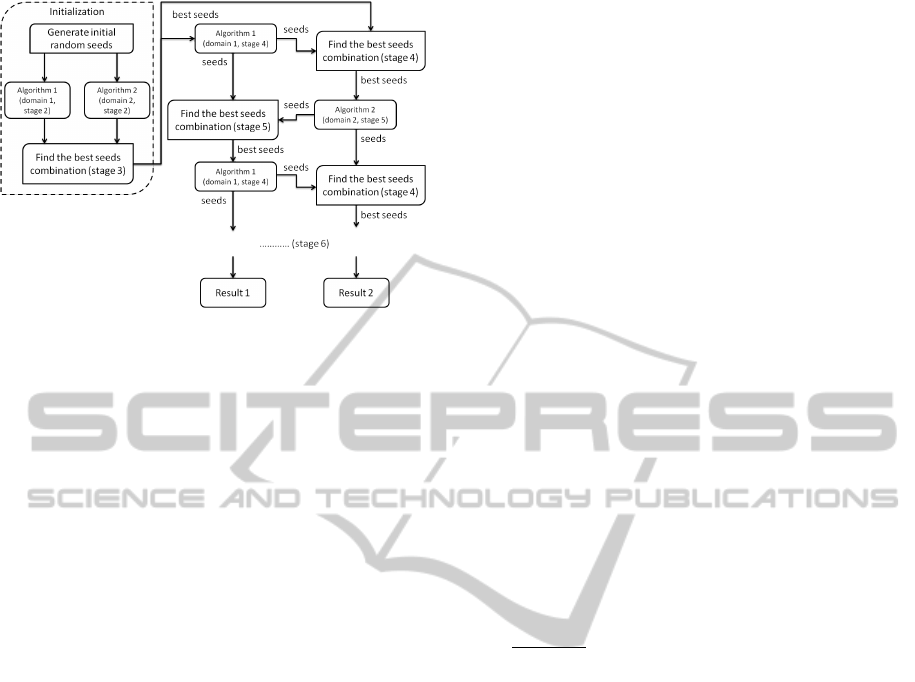
Figure 1: Overview of the semi-supervised seeding cluster-
ing approach.
without taking the sum over all centroids. To find
the best combination of centroids for domain T
1
,
we compare db
T
1
M
T
1
and db
T
1
M
T
2
for each centroid re-
sulting from clustering the data in domain T
1
and
resulting from clustering the data in domain T
2
,
and then take only those centroids which score a
lower value in the DB index, thus forming better
clusters in one domain compared to the other. We
then perform a similar operation for domain T
2
.
The outputs of this stage are two sets, each con-
sisting of the best combination of cluster centroids
or prototypes for each of the data domains T
1
and
T
2
, respectively.
4. In this stage, we use the best seeds obtained from
stage 3 to recompute the cluster centroids in the
first domain by running k-means for a small num-
ber (t
n
) of iterations; then compare these recom-
puted centroids against the cluster centroids that
were computed in the second domain in the previ-
ous iteration (as explained in detail in stage 3) and
find the best cluster centroids’ combination for the
second domain (T
2
).
5. Here, we use the best seeds obtained from stage 4
to initialize the k-modes algorithm in domain T
2
,
and run it for t
c
iterations. Then again, we com-
pare these recomputed centroids against the clus-
ter centroids computed in the first domain in the
previous iteration (as explained in detail in stage
3) and find the best cluster centroids’ combination
for the first domain (T
1
).
6. We repeat stages 4 and 5 until both algorithms
converge or the number of exchange iterations ex-
ceeds a maximum number. The general flow of
our approach is presented in Figure 1.
We compared the proposed mixed-type clustering
approach with the following two classical baseline ap-
proaches for clustering mixed numerical and categor-
ical data.
Baseline 1: Conversion: The first baseline ap-
proach is to convert all data to the same attribute type
and cluster it. We call this method the conversion al-
gorithm. Since we have attributes of two types, there
are two options to perform this algorithm:
1. Convert all numerical type attributes to categori-
cal type attributes and run k-modes.
2. Convert all categorical type attributes to numeri-
cal type attributes and run k-means.
Baseline 2: Splitting: The second classical base-
line approach is to run k-means and k-modes inde-
pendently on the numerical and categorical subsets of
attributes, respectively. We call this method the split-
ting algorithm.
The conversion algorithm requires data type con-
version: from numerical to categorical and from
categorical to numerical. There are several ways
to convert a numerical type attribute z, ranging in
[z
min
,z
max
], to a categorical type attribute y, also
known as “discretization” (Gan et al., 2007):
(i) by mapping the n numerical values, z
i
, to N
categorical values y
i
using direct categorization.
Then the categorical value is defined as y
i
=
b
N(z
i
−z
min
)
(z
max
−z
min
)
c + 1, where b c denotes the largest in-
teger less than or equal to z. Obviously, if z
i
=
z
max
, we get y
i
= N + 1, and we should set y
i
= N.
(ii) by mapping the n numerical values to N cate-
gorical values using a histogram binning based
method.
(iii) by clustering the n numerical values into N clus-
ters using any numerical clustering algorithm (e.g.
k-means). The optimal number of clusters N can
be chosen based on some validation criterion.
In the current implementation, we use cluster-based
conversion (iii) with the Silhouette index as a validity
measure because this results in the best conversion.
There are also several methods to convert categorical
type attributes to numerical type attributes:
(i) by mapping the n values of a nominal attribute
to binary values using 1-of-n encoding, result-
ing into transactional-like data, with each nominal
value becoming a distinct binary attribute
(ii) by mapping the n values of an ordinal nominal
attribute to integer values in the range of 1 to n,
resulting in numerical data with n values
(iii) without any mapping, but instead modifying our
distance measure so that for those nominal at-
tributes, a suitable deviation is computed (e.g. a
KDIR2012-InternationalConferenceonKnowledgeDiscoveryandInformationRetrieval
48
match between two categories results in a distance
of 0, while a non-match results in a maximal dis-
tance of 1). In this case, we need a clustering algo-
rithm that works on the distance matrix instead of
the input data vectors (also called relational clus-
tering ).
In our implementation, we used the first method (1-
of-n encoding).
3.2 The Case of a Different Number of
Clusters or Different Cluster
Partitions in each Data Type or
Domain
In our preliminary design above, the number of clus-
ters is assumed to be the same in each domain. This
can be considered as the default approach, and has the
advantage of being easier to design. However, in real
life data, there are two challenges:
• Case 1: The first challenge is when each data do-
main naturally gives rise to a different number of
clusters, which is simple to understand.
• Case 2: The second challenge is when regardless
of whether the number of clusters are similar or
different in the different domains, their nature is
actually completely different, and this will be il-
lustrated with the following example.
How do we combine the results of clustering in differ-
ent domains if the numbers of clusters are different?
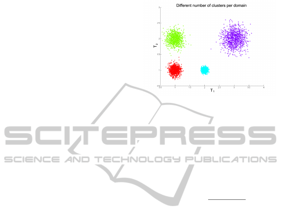
Let us look at the example shown in Figure 2, which
for visualization purposes, artificially splits the two
numerical features into two distinct domains, thus il-
lustrating the difficulties with mixed domains. Here
we have two domains or (artificially different) data
types T
1
and T
2
. In total, taking into account both
data domains or types T
1
and T
2
, we have four dis-
tinct clusters, however if we cluster each domain sep-
arately, we see that in T
1
, we have three clusters, while
in T
2
, we have only two clusters. This illustrates Case
2 and gives rise to the problem of judiciously combin-
ing the clustering results emerging from each domain
into a coherent clustering result with correct cluster
labelings for all the data points.
We propose the following algorithm to cluster
such a data set, that we emphasize, actually tar-
gets completely different data domains or types that
cannot be compared using traditional attribute-based
distance measures.
1. First, cluster T
1
with k
T
1
number of clusters and
cluster T
2
with k
T
2
number of clusters. Let M
T
1
be
the cluster membership matrix of domain T
1
and
M
T
2
be the cluster membership matrix of domain
Figure 2: Different number of clusters per domain.
T
2
. Therefore, M
T
1
is an n × k
T
1
matrix and M
T
2
is
an n × k
T
2
matrix, where n is the number of data
records. The membership matrix M
T
is such that
entry M
T
[i, j] is 1 or 0 depending on whether or
not point i belongs to cluster j in the current do-
main T .
2. Next, match each cluster j
1
in T
1
to the corre-
sponding cluster j
2
in T
2
. For this purpose, we
compute the Jaccard coefficient matrix J of size
k
T
1
× k
T
2
in which entry J[ j
1
, j
2
] is defined as fol-
lows:
J[ j
1
, j
2
] =
C
T
1
, j
1
∩C
T
2
, j
2
C
T
1
, j
1
∪C
T
2
, j
2
,
where C
T, j
is the set of points that belong to clus-
ter j in domain T , i.e.,
C
T, j
=
{
x
i
|M
T
(i, j) > 0
}
.
Then we compute the optimal cluster corre-
spondence using the Hungarian method with the
weight matrix W in which every entry, W[ j
1
, j
2
] =
1/J[ j
1
, j
2
] (Kuhn, 1955; Frank, 2005).
3. Finally, merge the clustering results of domains
T
1
and T
2
using Algorithm 1. Let T
max
be the do-
main with the highest number of clusters k
T
max
=
max{k
T
1
,k
T
2
} and M
T
max
be the membership ma-
trix of that domain. Let T
other
be the other domain
with a number of clusters k
T
other
(k
T
other
≤ k
T
max
)
and let its membership matrix be M
T
other
.
3.3 Computational Complexity
The complexity of the proposed approach is mainly
determined based on the complexity of the embed-
ded base algorithms used in each domain. In addi-
tion, there is the overhead complexity resulting from
the coordination and alternating seed exchange pro-
cess between the different domains during the mutual
supervision process. The main overhead computation
ASemi-supervisedLearningFrameworktoClusterMixedDataTypes
49

Algorithm 1 : Input: M
T
max
, M
T
other
, k
T
max
, th; Output:
M
merge
.
for j
1
= 1 to k
T
max
do
j
2
= argmax
j
2
[J
k
( j
1
, j
2
)]
C
T
max
, j
1
= {x
i
|M
T
max
(i, j
1
) > 0} {find points in
cluster j
1
in this domain}
C
T
other
, j
2
= {x
i
|M
T
other
(i, j
2
) > 0} {find points in
nearest cluster j
2
from other domain}
C
merge
= C
T
max
, j
1
∩C
0
T
other
, j
2
{find points in inter-
section between these two clusters}
if
|C
merge
|
|C
T
max
, j
1
|
> th then
C
new
= {x
i
|x
i
∈ C
merge
} {then assign intersec-
tion points to a new cluster}
C
T
max
, j
1
= C
T
max
, j
1
−C
new
{remove intersection
points from first cluster in this domain}
end if
end for
in the latter step is the cluster matching, validity scor-
ing and comparison performed in stage 3 (which is
then repeatedly invoked at the end of the subsequent
stages 4 and 5). Stage 3 involves the following com-
putations: first, the computation of the Jaccard coeffi-
cient matrix using the cluster memberships of the do-
mains in time O(k
2
N) (assuming the number of clus-
ters to be of similar order k), then, solving the cor-
respondence problem between the two domains us-
ing the Hunguarian method in time O(k
3
), and finaly,
computating of the DB indices for each cluster cen-
troid in both domains in time O(k
2
N). Thus, the to-
tal overhead complexity of stage 3 is O(k
2
N) since
k N. With the k-means and k-modes as the base
algorithms, the total computational complexity of the
proposed approach is O(N).
4 Experimental Results
4.1 Clustering Evaluation
The proposed semi-supervised framework was eval-
uated using several internal and external clustering
validity metrics. Note that in calculating all internal
indices that require a distance measure, we used the
square of the Euclidean distance for numerical data
types and the simple matching distance (Kaufman and
Rousseeuw, 1990) for categorical data types.
• Internal validity metrics
– The Davies-Bouldin (DB) index is a function
of the ratio of the sum of within-cluster scat-
ter to between-cluster separation (Davies and
Bouldin, 1979). Hence the ratio is small if the
clusters are compact and far from each other.
That is, the DB index will have a small value
for a good clustering.
– The Silhouette index is calculated based on
the average silhouette width for each sample,
average silhouette width for each cluster and
overall silhouette width for the entire data set
(Rousseeuw, 1987). Using this approach, each
cluster can be represented by its silhouette,
which is based on the comparison of its tight-
ness and separation. A silhouette value close to
1 means that the data sample is well-clustered
and assigned to an appropriate cluster. A sil-
houette value close to zero means that the data
sample could be assigned to another cluster,
and the data sample lies halfway between both
clusters. A silhouette value close to −1 means
that the data sample is misclassified and is lo-
cated somewhere in between the clusters.
– The Dunn index is based on the concept of clus-
ter sets that are compact and well separated
(Dunn, 1974). The main goal of this measure
is to maximize the inter-cluster distances and
minimize the intra-cluster distances. A higher
value of the Dunn index mean a better cluster-
ing.
• External validity metrics
– Purity is a simple evaluation measure that as-
sumes that an external class label is available to
evaluate the clustering results. First, each clus-
ter is assigned to the class which is most fre-
quent in that cluster, then the accuracy of this
assignment is measured by the ratio of the num-
ber of correctly assigned data samples to the
number of data points. A bad clustering has a
purity close to 0, and a perfect clustering has
a purity of 1. Purity is very sensitive to the
number of clusters, in particular, purity is 1 if
each point gets its own cluster (Manning et al.,
2008).
– Entropy is a commonly used information theo-
retic external validation measure that measures
the purity of the clusters with respect to given
external class labels (Xiong et al., 2006). A per-
fect clustering has an entropy close to 0 which
means that every cluster consists of points with
only one class label. A bad clustering has an
entropy close to 1.
– Normalized mutual information (NMI) esti-
mates the quality of the clustering with respect
to a groundtruth class membership (Strehl et al.,
2000). It measures how closely a clustering al-
gorithm could reconstruct the underlying label
KDIR2012-InternationalConferenceonKnowledgeDiscoveryandInformationRetrieval
50

Table 1: Data sets properties.
Data set No. of
Records
No. of Numerical
Attributes
No. of Categorical
Attributes
Adult 45179 6 8
Heart Disease Data 303 6 7
Credit Approval Data 690 6 9
distribution in the data. The minimum NMI is 0
if the clustering assignment is random with re-
spect to true class membership. The maximum
NMI is 1 if the clustering algorithm could per-
fectly recreate the true class memberships.
4.2 Equal Number of Clusters in each
Data Type or Domain
4.2.1 Real Data Sets
We experimented with three real-life data sets with
the characteristics shown in Table 1. All three data
sets were obtained from the UCI Machine Learning
Repository (Frank and Asuncion, 2010).
• Adult Data. The adult data set was extracted by
Barry Becker from the 1994 Census database. The
data set has two classes: People who make over
$50K a year and people who make less than $50K.
The original data set consists of 48,842 instances.
After deleting instances with missing and dupli-
cate attributes we obtained 45,179 instances.
• Heart Disease Data. The heart disease data, gen-
erated at the Cleveland Clinic, contains a mixture
of categorical and numerical features. The data
comes from two classes: people with no heart dis-
ease and people with different degrees of heart
disease.
• Credit Approval Data. The data set has 690 in-
stances, which were classified in two classes: ap-
proved and rejected.
4.2.2 Results with the Real Data Sets.
Since all three data sets have two classes, we clustered
them in two clusters.
1
We repeated each experiment
50 times (10 times for the larger adult data set), and
report the mean, standard deviation, minimum, me-
dian, and maximum values for each validation metric
(in the format of mean±std [ min, median, max ]).
• Adult Data: Table 2 shows the results of the adult
data set using the semi-supervised framework, the
conversion algorithm, and the splitting algorithm,
with the best results in a bold font. As the table
1
We realize the possibility of more than one cluster per
class, however we defer such an analysis to the future.
illustrates, the semi-supervised framework per-
forms better in both domains: showing significant
improvements in DB and Silhouette indices for
the numerical domain and almost all validity in-
dices for the categorical domain. Note the low
minimum value of the DB and high maximum
value of the Silhouette indices in the numerical
domain, showing that over all runs, the proposed
semi-supervised approach could achieve a better
clustering than classical baseline approaches.
• Heart Disease Data: Table 3 shows the results of
clustering the heart disease data set using the three
approaches. The conversion algorithms yielded
better clustering results for the numerical domain
based on the Dunn index and all external indices.
The semi-supervised approach outperforms the
conversion algorithm in the categorical domain
but conceded to the splitting algorithm.
• Credit Approval Data: Table 4 shows the results
of clustering the credit approval data set. Again,
the semi-supervised approach outperforms the tra-
ditional algorithms for the categorical type at-
tributes based on the internal indices but concedes
to the splitting algorithm in terms of all exter-
nal indices One possible reason is that the cluster
structure does not match the “true” class labels or
ground truth, which is common in unsupervised
learning. The splitting algorithms yielded better
clustering results for the numerical domain based
on the DB and Silhouette indices. Also note the
low minimum value of the DB and high maximum
value of the Silhouette indices in the numerical
domain for the semi-supervised approach, show-
ing that this approach can win by a large margin,
and this is one of the further areas of focus for our
ongoing work. Trying to reach these best results
in an unsupervised way.
4.3 Different Number of Clusters or
Different Cluster Partitions in each
Data Type or Domain
4.3.1 Data Sets
In the following experiments, as we have done with
our illustrating example above, we validate our sec-
ond algorithm on the data sets satisfying Case 2 (de-
scribed in Section 3.2) of non-coherent cluster parti-
tions across the different domains. Although in the
Iris data set, the attributes are of the same type, we
artificially split them into two domains so that we can
validate the method and visualize the input data and
the results. The validity of this example can general-
ASemi-supervisedLearningFrameworktoClusterMixedDataTypes
51

Table 2: Clustering result for the adult data set.
Algorithm Semi-supervised Conversion Splitting
Data type Numerical Categorical Numerical Categorical Numerical Categorical
DB Index 3.09 ±1.09[0.42,3.44,3.77] 1.22 ±0.14[1.10,1.12,1.40] 11.53 ±7.70[1.48,12.31,26.72] 1.50 ± 0.23[1.22,1.43, 1.92] 3.29 ± 0.001[3.29,3.29, 3.29] 1.15 ± 0.09[1.11,1.12, 1.37]
Silh. Index 0.29 ±0.18[0.18,0.21,0.71] 0.25 ±0.01[0.23,0.24,0.27] 0.07 ±0.05[−0.02,0.08,0.17] 0.22 ±0.02[0.19,0.21,0.25] 0.21 ±0.0[0.21,0.21,0.21] 0.25 ± 0.01[0.24,0.24, 0.27]
Dunn Index 1.1e − 4 ±4.2e − 4[1.2e − 5,1.2e − 5,1.1e − 3] 0.125 ±0.0[0.125,0.125,0.125] 0 ±0.00[0.00,0.00,0.00] 0.00 ± 0.00[0.00,0.00, 0.00] 0 ±0.00[0.00,0.00,0.00] 0.125 ± 0[0.125,0.125,0.125]
Purity 0.62 ±0.07[0.52,0.60,0.75] 0.59 ±0.06[0.50,0.56,0.67] 0.62 ±0.11[0.25,0.71,0.75] 0.56 ± 0.04[0.53,0.55, 0.65] 0.64 ± 0.001[0.64,0.64, 0.64] 0.59 ± 0.05[0.55,0.55,0.67]
Entropy 0.77 ± 0.03[0.72,0.78,0.79] 0.73 ±0.02[0.71,0.73,0.78] 0.73 ±0.06[0.69,0.69,0.81] 0.73 ± 0.02[0.70,0.74, 0.75] 0.71 ± 0.00[0.71, 0.71,0.71] 0.73 ± 0.01[0.71,0.73, 0.73]
NMI 0.06 ±0.03[0.02,0.05,0.10] 0.09 ±0.001[0.08,0.09,0.11] 0.08 ±0.07[2.1e− 4, 0.13,0.13] 0.09 ± 0.02[0.07,0.08, 0.12] 0.10 ± 0.00[0.10, 0.10,0.10] 0.09 ± 0.01[0.08,0.08, 0.11]
Table 3: Clustering result for the heart disease data set.
Algorithm Semi-supervised Conversion Splitting
Data type Numerical Categorical Numerical Categorical Numerical Categorical
DB Index 1.73 ±0.15[1.54, 1.71,2.14] 0.80 ±0.17[0.65, 0.77,1.42] 2.97± 0.56[0.21,2.95, 5.16] 1.13 ± 0.09[0.98,1.09, 1.35] 1.65 ±0.003[1.65, 1.65,1.65] 0.75 ±0.06[0.75, 0.75,0.77]
Silh. Index 0.33± 0.04[0.26, 0.33,0.41] 0.29± 0.02[0.23, 0.30,0.31] 0.26 ± 0.07[0.16,0.25, 0.75] 0.18 ±0.005[0.16, 0.18,0.19] 0.36 ±0.005[0.36, 0.36,0.36] 0.31 ±0.005[0.29, 0.31,0.31]
Dunn Index 3.3e −3 ± 2.2e − 3[1.2e − 5, 2.3e − 4, 0.35] 0.14 ± 0[0.14, 0.14,0.14] 0.04 ± 0.14[0.015, 0.015,0.98] 0.13 ± 0.04[0.07,0.15,0.23] 4.6e − 3 ±0[4.6e − 3,4.6e − 3,4.6e − 3] 0.14 ±0[0.14, 0.14,0.14]
Purity 0.72 ±0.03[0.65, 0.72,0.76] 0.78 ±0.03[0.71, 0.77,0.81] 0.77± 0.11[0.47,0.82, 0.82] 0.78 ± 0.02[0.75,0.76, 0.83] 0.75 ±0.003[0.75, 0.75,0.75] 0.81 ±0.01[0.78, 0.81,0.81]
Entropy 0.84 ±0.03[0.79, 0.84,0.91] 0.74 ±0.04[0.70, 0.75,0.87] 0.72± 0.11[0.67,0.67, 0.99] 0.74 ± 0.04[0.64,0.75, 0.81] 0.80 ±0.003[0.80, 0.80,0.81] 0.71 ±0.02[0.69, 0.69,0.76]
NMI 0.15 ±0.03[0.08, 0.16,0.20] 0.25 ±0.04[0.13, 0.24,0.30] 0.28 ± 0.11[2.1e − 4,0.32,0.32] 0.26 ± 0.04[0.18, 0.25,0.36] 0.19 ± 0.004[0.18,0.19, 0.19] 0.29± 0.02[0.23,0.30, 0.30]
Table 4: Clustering result for the credit card data set.
Algorithm Semi-supervised Conversion Splitting
Data type Numerical Categorical Numerical Categorical Numerical Categorical
DB Index 1.98 ±0.63[0.01,2.06,3.81] 1.41± 0.31[0.97,1.38, 1.95] 4.94 ±2.44[0.10, 4.87,8.57] 1.75 ± 0.22[1.32,1.69, 2.44] 1.89± 0.35[0.18, 1.97,1.97] 1.81 ±0.25[1.37,1.83,2.87]
Silh. Index 0.56 ±0.14[0.20,0.55,0.97] 0.23± 0.05[0.16,0.23, 0.36] 0.35 ±0.27[0.12, 0.29,0.92] 0.17 ± 0.02[0.13,0.16, 0.21] 0.63± 0.06[0.62, 0.62,0.95] 0.23 ±0.01[0.19,0.23,0.24]
Dunn Index 0.0078 ± 0.0497[1.2e −5, 2.3e − 4,0.35] 0.12 ± 0.03[0.11,0.11, 0.22] 0.06 ± 0.15[1.1e − 3, 0.011,0.77] 0.07 ± 0.002[0.07,0.07, 0.08] 0.003 ± 0.012[1.1e −4,1.1e − 4,0.06] 0.12 ± 0.01[0.11,0.12, 0.13]
Purity 0.65 ±0.05[0.47, 0.66,0.70] 0.73 ± 0.08[0.54,0.77, 0.80] 0.65± 0.12[0.48, 0.56,0.81] 0.77 ± 0.02[0.69,0.78, 0.82] 0.64± 0.02[0.56,0.64, 0.64] 0.79 ±0.01[0.76, 0.79,0.82]
Entropy 0.91 ±0.04[0.84,0.91,0.99] 0.80± 0.08[0.70,0.78, 0.98] 0.86 ±0.13[0.68, 0.97,0.99] 0.77 ± 0.03[0.67,0.76, 0.87] 0.93± 0.01[0.93, 0.93,0.98] 0.73 ±0.02[0.65,0.73,0.78]
NMI 0.10 ±0.04[1.3e− 4, 0.09,0.18] 0.19 ±0.08[0.01, 0.22,0.30] 0.13 ± 0.13[1.2e − 4,0.03, 0.31] 0.23 ±0.03[0.12, 0.23,0.31] 0.08 ± 0.01[0.03,0.08, 0.08] 0.26± 0.02[0.22, 0.27,0.36]
Table 5: Basic characteristics of the Iris data set.
Attribute Min Max Mean Standard deviation Class Correlation (Pearson‘s CC)
Sepal length 4.3 7.9 5.84 0.83 0.7826
Sepal width 2.0 4.4 3.05 0.43 −0.4194
Petal length 1.0 6.9 3.76 1.76 0.9490
Petal width 0.1 2.5 1.20 0.76 0.9565
Table 6: Overview of the experiments.
Experiment Number Data set T
1
T
2
k
T
1
k
T
2
K Threshold
1 Iris {1} {3} 2 3 3 0.6
2 Iris {2} {4} 2 3 3 0.6
3 Iris {1, 3} {2, 4} 2 3 3 0.6
ize for different domains, because we do not exploit
any attribute-based distance measure between the dif-
ferent data domains (as would be the case for really
different domains). The Iris data set is a benchmark
set that contains 3 classes of 50 data instances each,
where each class refers to a type of iris plant: iris Se-
tosa, iris Versicolour, iris Virginica.
4.3.2 Experiments
All three experiments were performed on the Iris data
set. We repeated each experiment 10 times and re-
port only the best results. For validation purposes, we
used the class labels. For class - cluster assignment
we used the Jaccard coefficient, meaning that a class
will be assigned to the cluster with highest Jaccard
coefficient.
Experiment 1. We first take only the first and third
features of the IRIS data set. Let T
1
be the sepal length
(first feature) and T
2
be the petal length (third feature).
Table 7: Experiment 1: Evaluation measures for the semi-
supervised merging algorithm and k-means (bold results are
best).
Algorithm Class Precision Recall F-measure Accuracy Purity Entropy NMI
K-means
Setosa 0.9804 1.0 0.9901 0.9933
0.8800 0.2967 0.7065
Versicolour 0.7758 0.9 0.8333 0.88
Virginica 0.9224 0.74 0.8132 0.8868
Semi-supervised merging
Setosa 1.0 1.0 1.0 1.0
0.9467 0.1642 0.8366
Versicolour 0.8889 0.96 0.9231 0.9467
Virginica 0.9565 0.88 0.9167 0.9467
We chose those two features because the first feature
has a low class correlation index while the third fea-
ture has a high class correlation index. The first ex-
periment was performed in the following steps:
1. Cluster the data in domain T
1
using k-means
(k = 2)
2. Cluster the data in domain T
2
using k-means
(k = 3)
3. Merge the two clustering results using the merg-
ing algorithm described in Algorithm 1. Notice
that one of the output parameters is K, which is
the number of clusters after merging. We set the
overlap threshold parameter to th = 0.6.
4. Compare this result with the clustering result of
k-means using k = K clusters, performed on do-
mains T
1
and T
2
together.
Table 7 shows the results in terms of classification ac-
curacy, precision, recall, F-measure, purity, entropy
and NMI for each algorithm (the results in bold are
better).
Experiment 2. We next performed a similar exper-
iment to the above but this time, domain T
1
is the 2nd
KDIR2012-InternationalConferenceonKnowledgeDiscoveryandInformationRetrieval
52

feature - sepal width, while T
2
is the 4th feature - petal
width. The overlap threshold was set to th = 0.6. On
the Table 8 shown the results for the second experi-
ment in terms of relevance measures.
Experiment 3. We repeated the same experiment as
above, but this time, domain T
1
consists of the 1st and
3rd features, while T
2
consists of the 2nd and 4th fea-
tures. The overlap threshold was set to th = 0.6. The
results of the second experiment are shown in Table
9.
Table 8: Experiment 2: Evaluation measures for the semi-
supervised merging algorithm and k-means (bold results are
best).
Algorithm Class Precision Recall F-measure Accuracy Purity Entropy NMI
K-means
Setosa 1.0 0.98 0.9899 0.9933
0.9268 0.2265 0.7738
Versicolour 0.8679 0.92 0.8932 0.9267
Virginica 0.9167 0.88 0.8979 0.9333
Semi-supervised merging
Setosa 1.0 1.0 1.0 1.0
0.9600 0.1360 0.8642
Versicolour 0.9231 0.96 0.9412 0.96
Virginica 0.9583 0.92 0.9388 0.96
Table 9: Experiment 3: Evaluation measures for the semi-
supervised merging algorithm and k-means (bold results are
best).
Algorithm Class Precision Recall F-measure Accuracy Purity Entropy NMI
K-means
1 - Setosa 1.0 1.0 1.0 1
0.8933 0.2485 0.7582
2 - Versicolour 0.7742 0.96 0.8574 0.8933
3 - Virginica 0.9474 0.72 0.8182 0.8933
Semi-supervised merging
1 - Setosa 1.0 0.98 0.9899 0.9933
0.9267 0.2265 0.7738
2 - Versicolour 0.86792 0.92 0.8932 0.92667
3 - Virginica 0.9167 0.88 0.8980 0.9333
4.3.3 Results with the IRIS Data Set
In the first and second experiments, the semi-
supervised merging algorithm outperformed the k-
means algorithm. In the third experiment, the merg-
ing algorithm obtained similar results to the k-means
algorithm, although it still outperformed the k-means
in terms of the purity of the results and giving a lower
entropy of the clustering overall.
5 CONCLUSIONS
The results of our preliminary study show that the
proposed semi-supervised framework tends to yield
better clustering results in the categorical domain.
Thus the seeds obtained from clustering the numer-
ical domain tend to provide additional helpful knowl-
edge to the categorical clustering algorithm (in this
case, the K-modes algorithm). This information is
in turn used to avoid local minima and obtain a bet-
ter clustering in the categorical domain. We are cur-
rently completing our study by (1) extending our ex-
periments and methodology to mixed data involving
transactional information (particularly text and click-
streams) as one of the types, and (2) devising a suit-
able method for further combining the results of the
multiple clusterings performed on each data type or
domain. This is because, although each one of the
data type-specific algorithms receives some guidance
from the algorithm that clustered the other data types,
the final results are currently not combined, but are
rather still being evaluated in each domain separately.
One promising direction is to combine the multiple
clustering results such that the best clustering deci-
sions are selected (or merged) from each result. A
challenging issue is whether to merge decisions at the
cluster prototype/parameter level or at the data parti-
tioning/labeling level, or both. We are also extending
our technique so that the number of clusters is allowed
to vary from one domain (or attribute type) to another.
ACKNOWLEDGEMENTS
This work was supported by US National Science
Foundation Data Intensive Computation Grant IIS-
0916489.
REFERENCES
Al-Razgan, M. and Domeniconi, C. (2006). Weighted clus-
tering ensembles. In Proc. of the 6th SIAM ICML.
Banerjee, A., Dhillon, I. S., Ghosh, J., Sra, S., and Ridge-
way, G. (2005). Clustering on the unit hypersphere
using von mises-fisher distributions. Journal of ML
Research, 6.
Basu, S., Banerjee, A., and Mooney, R. (2002). Semi-
supervised clustering by seeding. In Proc. of 19th
ICML.
Blum, A. and Chawla, S. (2001). Learning from Labeled
and Unlabeled Data Using Graph Mincuts. In Proc.
18th ICML, pages 19–26.
Blum, A. and Mitchell, T. (1998). Combining labeled and
unlabeled data with co-training. In Proc. of the 11th
annual conference on CL theory, pages 92–100.
Cohn, D., Caruana, R., and Mccallum, A. (2003). Semi-
supervised clustering with user feedback. Technical
report.
Davies, D. L. and Bouldin, D. W. (1979). A cluster sepa-
ration measure. Pattern Analysis and Machine Intelli-
gence, pages 224 –227.
Dhillon, I. S. and Modha, D. S. (2001). Concept decom-
positions for large sparse text data using clustering.
Mach. Learn., 42:143–175.
Dunn, J. C. (1974). Well separated clusters and optimal
fuzzy partitions. J. Cybern, 4:95–104.
Ester, M., peter Kriegel, H., S, J., and Xu, X. (1996).
A density-based algorithm for discovering clusters in
large spatial databases with noise. In Proc. of the Sec-
ond International Conference on KDD, pages 226–
231.
ASemi-supervisedLearningFrameworktoClusterMixedDataTypes
53

Frank, A. (2005). On kuhn’s hungarian method - a tribute
from hungary. Naval Research Logistics (NRL), 52:2–
5.
Frank, A. and Asuncion, A. (2010). UCI machine learning
repository.
Gan, G., Ma, C., and Wu, J. (2007). Data Clustering: The-
ory, Algorithms, and Applications. Society for Indus-
trial and Applied Mathematics.
Ganti, V., Gehrke, J., and Ramakrishnan, R. (1999). Cactus
- clustering categorical data using summaries. In Proc.
of the 5th ACM SIGKDD International Conference on
KDD, pages 73–83.
Ghaemi, R., Sulaiman, M. N., Ibrahim, H., and Mustapha,
N. (2009). A survey: Clustering ensembles tech-
niques.
Guerrero-Curieses, A. and Cid-Sueiro, J. (2000). An en-
tropy minimization principle for semi-supervised ter-
rain classification. In Image Processing, 2000 Inter-
national Conference on, volume 3, pages 312 – 315.
Guha, S., Rastogi, R., and Shim, K. (2000). Rock: A robust
clustering algorithm for categorical attributes. Infor-
mation Systems, 25:345 – 366.
Huang, Z. (1997). A fast clustering algorithm to cluster
very large categorical data sets in data mining. In In
Research Issues on KDD, pages 1–8.
Huang, Z. (1998). Extensions to the k-means algorithm for
clustering large data sets with categorical values. Data
Mining and Knowledge Discovery, 2:283–304.
Joachims, T. (1999). Transductive inference for text clas-
sification using support vector machines. In Proc. of
16th ICML, pages 200–209, Bled, SL.
Karypis, G. and Kumar, V. (1998). A fast and high qual-
ity multilevel scheme for partitioning irregular graphs.
SIAM Journal on Scientific Comp., 20(1):359–392.
Kaufman, L. and Rousseeuw, P. (1990). Finding Groups in
Data An Introduction to Cluster Analysis.
Kuhn, H. W. (1955). The hungarian method for the assign-
ment problem. Naval Research Logistic Quarterly,
2:83–97.
MacQueen, J. B. (1967). Some methods for classification
and analysis of multivariate observations. In Proc. of
the 5th Berkeley Symposium on Math. Statistics and
Probability, volume 1, pages 281–297.
Manning, C. D., Raghavan, P., and Schtze, H. (2008). In-
troduction to Information Retrieval.
Nigam, K., McCallum, A. K., Thrun, S., and Mitchell, T.
(2000). Text classification from labeled and unlabeled
documents using em. Mach. Learn., 39:103–134.
Plant, C. and Böhm, C. (2011). Inconco: interpretable clus-
tering of numerical and categorical objects. In Proc.
of the 17th ACM SIGKDD International Conference
on KDD, pages 1127–1135.
Rousseeuw, P. (1987). Silhouettes: a graphical aid to the in-
terpretation and validation of cluster analysis. J. Com-
put. Appl. Math., 20:53–65.
Shi, J. and Malik, J. (2000). Normalized cuts and image
segmentation. IEEE Transactions on Pattern Analysis
and Machine Intelligence, 22(8):888–905.
Strehl, A., Strehl, E., Ghosh, J., and Mooney, R. (2000).
Impact of similarity measures on web-page clustering.
In Workshop on AI for Web Search, pages 58–64.
Wagstaff, K., Cardie, C., Rogers, S., and Schrödl, S.
(2001). Constrained k-means clustering with back-
ground knowledge. In Proc. of the 18th ICML, pages
577–584.
Xiong, H., Wu, J., and Chen, J. (2006). K-means clus-
tering versus validation measures: a data distribution
perspective. In Proc. of the 12th ACM SIGKDD inter-
national conference on KDD, pages 779–784.
Zeng, H.-J., Wang, X.-H., Chen, Z., Lu, H., and Ma, W.-
Y. (2003). Cbc: clustering based text classification
requiring minimal labeled data. In Data Mining, Third
IEEE ICDM, pages 443 – 450.
Zhong, S. (2006). Semi-supervised model-based document
clustering: A comparative study. Mach. Learn., 65:3–
29.
Zhong, S. and Ghosh, J. (2003). A unified framework
for model-based clustering. Journal of ML Research,
4:1001–1037.
Zhu, X., Ghahramani, Z., and Lafferty, J. (2003). Semi-
supervised learning using gaussian fields and har-
monic functions. In Proc. 20th International Conf.
on ML, pages 912–919.
KDIR2012-InternationalConferenceonKnowledgeDiscoveryandInformationRetrieval
54
