
User based Collaborative Filtering with Temporal Information for
Purchase Data
Maunendra Sankar Desarkar and Sudeshna Sarkar
Department of CSE, Indian Institute of Technology Kharagpur, Kharagpur, India
Keywords:
Item Recommendation, Collaborative Filtering, Temporal Recommendation.
Abstract:
User based collaborative filtering algorithms are widely used for generating recommendations for users. Stan-
dard user based collaborative filtering algorithms do not consider time as a factor while measuring the user
similarities and building the recommendation list. However, users’ interests often shift with time. Recom-
mender systems should therefore rely on recent purchases of the users to address this user dynamics. Items
also have their own dynamics. Most of the items in a recommender system are widely popular just after their
releases butdo not sell that well afterwards. Giving more importance to the recent purchases of the experts may
capture the item dynamics and hence result in better recommendation accuracy. We study the performances
of different time-aware user based collaborative filtering algorithms on several benchmark datasets. The pro-
posed algorithms use the time-of-purchase information for calculating user similarities. The time information
is also used while combining the purchase behaviors of the experts and generating the final recommendation.
1 INTRODUCTION
In the recommendation problem, given a set of pur-
chase records from different users, the task is to find
a list of recommended or suggested items for the
users. This list of items would be different for dif-
ferent users, as each user has his/her own personal
choices of the items.
Users’ purchase patterns for different products
are different. For systems where a user may pur-
chase/access the same item multiple times (e.g.
music/video/article hosting systems, stores selling
household items), past purchases by a user can be
used as a basis for future recommendation. On the
other hand, there are systems where the user gener-
ally does not purchase the same item more than once.
Examples include purchases of books, music CDs,
Movie DVDs etc. In such cases, the system can con-
sider purchases or accesses made by users with sim-
ilar purchase or access behaviors. User based col-
laborative filtering algorithms that use this concept of
similar tastes of users can be used for recommending
items for purchase stores where the same user does
not purchase the same item more than once.
Traditional user based collaborative filtering algo-
rithms do not consider time as a factor while finding
similar users and generating the recommendation list.
The basic user based collaborative filtering frame-
work may not work well if the interest profile of the
user changes with time. In reality, users’ interests of-
ten shift over time. If the algorithm looks at the entire
purchase history of the user, and gives equal impor-
tance to all the items purchased in the past, the rec-
ommended list may include items that are much sim-
ilar to the ones the user liked in the past. Chances
are that the user will not like those items as his inter-
est has now shifted to different types of items. Such
situations may be addressed by focusing more on the
recent purchases of the users.
The items also have their own dynamics. Many
items are popular in a narrow time window after their
release. As the time progresses, their purchases de-
crease, and after some time, the item is not purchased
much. The length of this window (which we call pop-
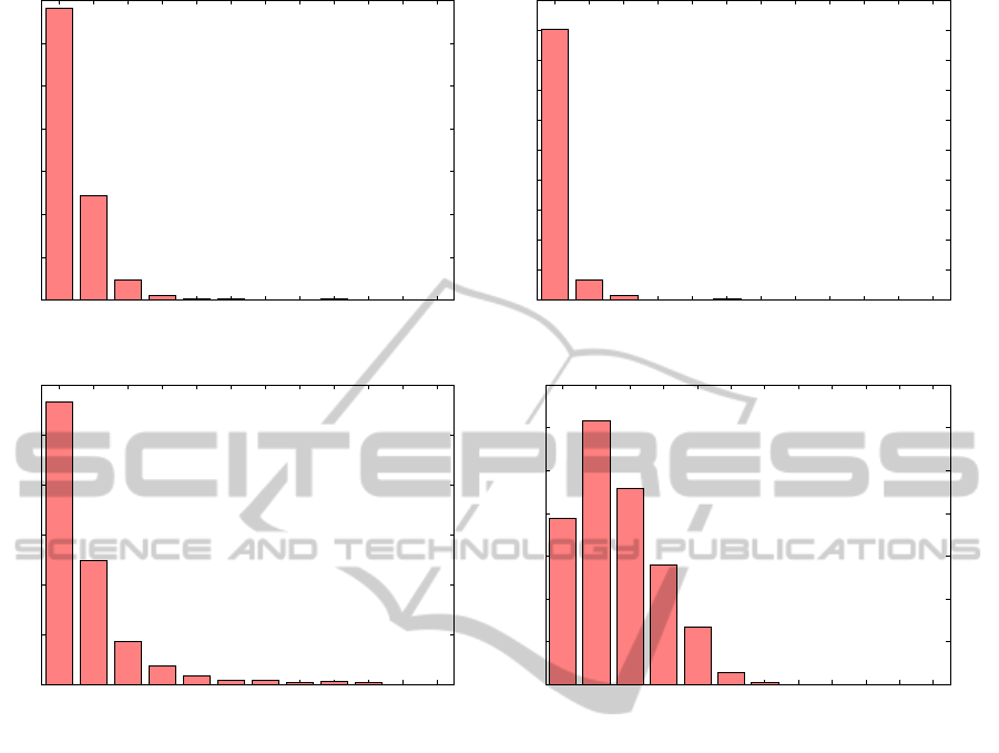
ularity span) may vary from item to item. We looked
at the popularity spans of different items from sevaral
real world datasets. It was observed that, for all the
datasets, the popularity of majority of the items decay
with time. Figure 1 shows the popularity span his-
togram for sample datasets from Amazon and Netflix.
One can use the information regarding the current
selling trend of the items while generating the recom-
mendations. If an item is currently popular, the item
can be recommended to many users. However, if a
system recommends items by looking at the popular-
ity value only, then the recommendation will lose the
55
Desarkar M. and Sarkar S..
User based Collaborative Filtering with Temporal Information for Purchase Data.
DOI: 10.5220/0004134400550064
In Proceedings of the International Conference on Knowledge Discovery and Information Retrieval (KDIR-2012), pages 55-64
ISBN: 978-989-8565-29-7
Copyright
c
2012 SCITEPRESS (Science and Technology Publications, Lda.)
0
0.1
0.2
0.3
0.4
0.5
0.6
0.7
10 20 30 40 50 60 70 80 90 100 110 120
(a) Item popularity span histogram for Amazon Music dataset
0
0.1
0.2
0.3
0.4
0.5
0.6
0.7
0.8
0.9
1
10 20 30 40 50 60 70 80 90 100 110 120
(b) Item popularity span histogram for Amazon DVD dataset
0
0.1
0.2
0.3
0.4
0.5
0.6
10 20 30 40 50 60 70 80 90 100 110 120
(c) Item popularity span histogram for Amazon Book dataset
0
0.05
0.1
0.15
0.2
0.25
0.3
0.35
10 20 30 40 50 60 70 80 90 100 110 120
(d) Item popularity span histogram for Netflix dataset
Figure 1: Item popularity span histograms for different datasets. For each dataset, we considered the items that were purchased
at least 20 times. If the popularity score of an item i in month m is at least 20, then we say that the product was popular in
month m. The largest popularity span of an item is the largest time window (in months) in which the item was popular. Each
graph represents the histogram of the largest popularity span for different items in a particular dataset. Y-axis shows the
fraction of items that fall in a particular bin of the histogram.
personalization aspect. The system may recommend
an item just because it is popular,but the user may not
have any interest in that item. On the other hand, for a
target user u, if an item is popular among many of the
users who have interests similar to that of u, then the
item might be of interest to u also. We try to incorpo-
rate the item dynamics in the user based collaborative
filtering framework by looking at the recent purchases
of the similar users or experts.
In this work, we explore several time-aware user
based collaborativefiltering algorithms for the recom-
mendation problem on purchase data. We perform
experimentation on Amazon and Netflix datasets and
analyze the performances of the algorithms. We con-
duct experiments in a framework where the recom-
mendation algorithms are run just prior to each pur-
chase made by the user, and we see if the system is
able to include the next purchase in its recommen-
dation list. Experimental results indicate that recom-
mendation performance can be improved by giving
more importance to the recent purchases of both the
user and the experts.
2 RELATED WORK
There has been some research work on designing
time-aware collaborative filtering algorithms for solv-
ing the recommendation problem. (Kawamae et al.,
2009) considers precedence information at user level
and uses it for recommendation generation. A user
who not only purchases many of the items that the
target user also purchases, but also makes those pur-
chases before the target user can be used as an expert
for recommending items to the target user. It also con-
siders other time specific factors such as launch time
of items in the recommendation model. In (Lee et al.,
KDIR2012-InternationalConferenceonKnowledgeDiscoveryandInformationRetrieval
56

2008), the authors proposed an algorithm that con-
verts a purchase to an implicit rating by considering
the launch-time of the item and the time of the pur-
chase. This implicit rating is then used in collabora-
tive filtering framework for recommendation. A rec-
ommender system based on tag and time information
for social tagging systems is presented in (Zheng and
Li, 2011). It uses a combination of a tag-weight ma-
trix and a time-weight matrix for this purpose. For
each user-tag pair, the tag-weight matrix stores the
fraction of times the user has used the tag. The time-
weight matrix, for a user-tag pair, stores a value that is
dependent on the time when the user entered the tag.
Temporal algorithms have also been used for solv-
ing various other types of recommendation problems.
In (Parameswaran et al., 2010), the authors propose a
precedence mining model that estimates the probabil-
ity of future consumption based on temporal patterns.
The algorithm is used for a course recommendation
application where depending on the past courses that
a student has taken new courses are suggested to the
student. There are algorithms that study temporal-
ity where there is a strict order or path followed by
the user, and the goal is to predict the next step in
that sequence. A typical example of such a task is
the next-page prediction problem in which the system
tries to predict the next web page a user will access
given a sequence of pages visited up to now ((Desh-
pande and Karypis, 2004)). In (Shani et al., 2005),
purchase sequences are viewed as states of a dynamic
system. If one sequence leads to another sequence,
then the system is considered to have made a transi-
tion to the new state. This state transition model is
described as a Markov Decision Process and is used
to generate recommendations. Algorithms based on
precedence mining may not be appropriate for solving
the recommendation problem in a more general case
where such precedence information are not much use-
ful. Two users who purchase the same set of products,
but in different order, may have similar tastes of the
items. One of these users can be used for generating
recommendations for the other. (Rendle et al., 2010)
uses a matrix factorization technique over personal-
ized Markov chains representing sequential purchase
patterns of users. This method called FPMC (Fac-
torizing Personalized Markov Chains) is used for the
next basket recommendation problem. The method
assumes that a user may purchase the same item mul-
tiple times.
A related problem where time aware algorithms
have also been used is the rating prediction problem.
Rating prediction problem is used in systems where
users give ratings to different items. In (Ding and
Li, 2005; Ding et al., 2006), the authors assign time
weights for items so that the recently rated items are
able to contribute more to the prediction. (Campos
et al., 2010) calculates the most similar users with all
the available information from the dataset. After that,
only the most recent ratings of the neighbors are used
to find the predicted rating. (Koren, 2008) merges the
factor and neighborhood models for collaborative fil-
tering to solve the task of rating prediction. A factor
model that looks at several temporal aspects from rat-
ing data is discussed in (Koren, 2009).
A combination of bias model and time weighted
similarity model is presented in (Rongfei et al., 2010).
3 PRELIMINARIES AND
PROBLEM DEFINITION
Let U and I be the set of users and items respectively.
Let D be a collection of past purchase records. Each
record in D is called a purchase or a transaction, and
is of the form (u,i,t
ui
) which represents the fact that
user u has purchased item i at time t
ui
.
Given a target user u ∈ U and past purchase data
D, the goal of a recommender system is to find a set
R
u
⊆ I of items that the target user may want to pur-
chase in future.
4 OUR ALGORITHMS
For the systems where the same users generally do
not purchase the same items multiple times, the user
based collaborativefiltering frameworkis widely used
for generating the recommendations. Algorithms us-
ing this framework work in two phases: expert selec-
tion and recommendation generation. As discussed in
Section 1, giving importance to the recent purchases
of the user in the expert selection phase may address
the issues related to the users’ interest shift. Giving
more importance to the recent purchases of the ex-
perts may capture the item dynamics. For both the
target user and the experts, the system can look at
their purchase histories in three different ways: (a)
treat all items as equal, (b) consider items purchased
in a small time window, or (c) look at the entire his-
tory but with discounted importance assigned to the
items purchased long back. We explore four out of
these nine different combinations and present those
algorithms in this section.
4.1 Algorithm 1: Count (CNT)
The first among these four algorithms does not look
at time information. We call this algorithm as Count,
UserbasedCollaborativeFilteringwithTemporalInformationforPurchaseData
57

or CNT in short. We use this algorithm as the base-
line. We estimate the Similarity weight of a user v for
a target user u as the number of items that both u and
v have purchased
1
. The top-K users according to the
similarity weights are selected as the experts. In the
second phase, the algorithm looks at the purchase his-
tories of the experts. For each item, its score is given
by the number of experts who have purchased it. The
items are then sorted in non-increasing order of their
scores, and the top N items are recommended to u.
4.2 Algorithm 2: Recent-k (RECK)
CNT looks at all the purchases made by the users in
the past and treats them equally. However, users’ in-
terests often shift over time. To handle this situation,
we do not look at the entire history of the target user’s
purchases. Our next algorithm RECK looks at a small
window (say, of size k) of his/her recent purchases.
Experts are selected based on how many of the items
from this window they have bought.
Let the set of the k most recent purchases of user
u be I
k
u
. The expert selection and recommendation
generation phases are performed as follows:
• For each user v ∈ U \ i, find weight w
v
=
|I
k
u
T
I
v
|. Select top-K experts according to sim-
ilarity weights. Let this set be E.
• For each item i /∈ I
u
, score s
i
=
∑
v∈E∧i∈I
v
w
v
. Rec-
ommend top-N items with the highest scores.
4.3 Algorithm 3: Recent-k with Weight
(RECKW)
The next algorithm, represented by RECKW, extends
RECK by adding more time-dependent factors in the
expert selection and recommendation generation pro-
cesses. RECK looks at only the most recent purchases
of the target user to find the experts. In RECK, if v
purchased many items that the target user u has pur-
chased recently, then v gets high similarity weight for
u. However, all those purchases of v might be made
long back. If this user v is selected as an expert,
and v’s interest has shifted recently, then the system
may end up recommending many items that v has pur-
chased recently, but those items do not match u’s re-
cent taste. This observation motivated us to look at v’s
recent interest, and give more weight to v if his/her re-
cent purchases are similar to u’s recent purchases. To
calculate the item’s contribution to the user’s similar-
ity weight, we take help of a decay function that we
denote by decay(t). There are two properties that the
1
Please note that the it is not necessary to normalize the
similarity weights in a fixed range.
function should have: (a) It should be monotonically
decreasing, and (b) for very large values oft, the value
of the function should be small but non-zero. The first
property ensures that recent purchases are more im-
portant than old purchases. The second property sig-
nifies that very old purchases are not completely ig-
nored, but they have much lesser importance weight
compared to recent purchases. We use the following
decay function in our algorithms.
decay(t) =
γ
t
+ λ
1+ λ
. (1)
γ and λ are constants and assume values from the
continuous interval [0,1]. It can be easily verified that
the function is monotonically decreasing. Also, for
very large t, the value of the function is
λ
1+λ
, which is
non zero. This value can be controlled by choosing a
value of λ that is suitable for the application. Hence,
the function satisfies the above properties. Please note
that there are several different choices of decay func-
tions. However, our focus in this work is to show that
recommendation performances can be improved by
giving more importance on the users’ and the experts’
recent purchases. So we chose a function that satis-
fies above two properties and used it for generating
recommendations. We did not do much experimenta-
tion regarding different forms of decay functions.
The steps used by RECKW for expert selection
is similar to the steps used in RECK. The only dif-
ference is that each item in C = I
k
u
T
I
v
now con-
tributes decay(τ − t
vi
) to v’s similarity weight, where
τ is the current time. So, items recently purchased by
v are given more importance. In the second phase,
for each item i ∈ I
v
, expert v contributes a score of
w
v
∗ decay(τ − t
vi
). The scoring rule suggests that if
there are many products that an expert has purchased,
then the ones that are purchased more recently will
get higher score. The top-N items with the highest
score are recommended to the target user. The basic
steps of the algorithm are outlined below:
• For each user v ∈ U \ u, find the co-purchased
items C = I
k
u
T
I
v
.
• Set v’s weight w
v
=
∑
|C|
j=1
decay(τ−t
vC( j)
). Select
top-K users (E) as experts.
• For each item i /∈ I
u
, set score s
i
=
∑
v∈E∧i∈I
v
w
v
∗
decay(τ−t
vi
). Output top-N items as recommen-
dations.
4.4 Algorithm 4: Entire History with
Discounted Weight (DISCHIST)
RECK and RECKW look at k most recent purchases of
the target user u. Though the most recent purchases
KDIR2012-InternationalConferenceonKnowledgeDiscoveryandInformationRetrieval
58

of a user are perhaps the most important and represen-
tative of the user’s recent interest, the past purchases
may not be totally unimportant. For users whose in-
terests have remained the same over long periods of
time, looking at some more purchases from the past
may be useful. We wanted to see if we can im-
prove the performance of recommendation by look-
ing at all past purchases of u. However, treating all
past purchases equally may decrease the performance
of the algorithm for those users whose interests have
changed over time. To avoid such a scenario, we
use the concept of importance weight, where recent
purchases are given more weight but old purchases
are given less, but non-zero weight. The importance
weight may be characterized by a decay function as
defined in Equation 1. In algorithm DISCHIST, each
purchase of user u of the form (u,i,t
ui
) is assigned an
importance weight of decay(τ − t
ui
), where τ is the
current time. As the decay function is monotonically
decreasing in nature, users who have purchased many
of the items that u has purchased recently get higher
weight than those who have purchased many items
that u had purchased long back. The rest of the steps
are similar to that in RECKW. A brief outline of the
steps are given below.
• For each user v ∈ U \ u, find the co-purchased
items C = I
u
T
I
v
.
• Set v’s weight w
v
=
∑
|C|
j=1
decay(τ−t
uC( j)
). Select
top-K users (E) as experts.
• For each i /∈ I
u
, set score s
i
=
∑
v∈E∧i∈I
v
w
v
∗
decay(τ−t
vi
). Output top-N items as recommen-
dations.
5 EXPERIMENTAL RESULTS
5.1 Datasets Used
We used the Amazon product co-purchase metadata
2
and a sample of the Netflix data
3
for comparative
evaluation of the recommendation algorithms. The
Amazon dataset contains details of different products
sold on amazon. The products are of five types: Book,
Music, DVD, Video and Toy. There were not many
products for the “Toy” and “Video” categories. We
used the data for Music, DVD and Book categories
for experimentation.
There are not many publicly available datasets
for evaluating product recommendation algorithms.
2
http://snap.stanford.edu/data/amazon-meta.html
3
http://www.netflixprize.com/
However, several datasets are available for evaluat-
ing rating prediction algorithms. We use one such
dataset, the Netflix dataset, for for our experiments.
In the Netflix dataset, users rate different movies that
they have rented. If a user has rated a movie in this
dataset, then it can be assumed that the user was in-
terested in watching the movie. Hence if a recom-
mender system could recommend that movie just be-
fore the user decided the watch the movie, the user
could have accepted the recommendation. Based on
this intuition, we converted the Netflix dataset into a
purchase dataset. If a user has rated a movie, then we
assume that the user has rented/purchased the movie.
In (Kawamae et al., 2009), the authors used the Net-
flix dataset for evaluating the proposed recommenda-
tion generation algorithm.
5.2 Preprocessing the Datasets
For each product, the Amazon dataset mentions its
product type, different categories that the product be-
longs to, and a list of reviewers who have reviewed
the product. In most cases, a user reviewed a product
only once. We considered these reviews as purchases.
i.e., if user u has reviewed item i, we considered that
u has purchased i. Also, for each review, the dataset
mentions the date on which the review was entered. If
user u has entered multiple reviews for product i, then
we keep the earliest review and remove the rest from
the dataset. We separated out data for each differ-
ent product type from the dataset. So, we used three
different datasets for the Amazon data, for the three
different product categories namely Book, Music and
DVD.
For the Netflix dataset, the sample was taken by
considering the first 1500movies as items and the per-
sons who have rated those movies as users. If a user
had rated a movie, we consider that the user has pur-
chased the movie. In the Netflix dataset, each user
rates a movie at most once.
For both Amazon and Netflix datasets, we re-
moved from the datasets any transaction correspond-
ing to a user with fewer than m
l
total purchases. This
preprocessing enabled us to remove some of the non-
prolific users. Also, we removed from the dataset
transactions corresponding to users who made more
than m
u
purchases. This was necessary so that we
could fit the co-purchase network (as mentioned in
Section 5.5) in the memory. For the Amazon datasets
(Book, Music and DVD), values of m
l
and m
u
were
set to 50 and 200 respectively. For the Netflix dataset,
m
l
and m
u
were fixed at 20 and 400 respectively. For
all datasets, time information was maintained in unit
of months.
UserbasedCollaborativeFilteringwithTemporalInformationforPurchaseData
59

Table 1: Summary comparison of the algorithms. C is the items of importance. E is the set of experts. w
v
is the weight of user
v as computed during the expert selection phase. s
i
is the score of item i as computed in recommendation generation phase.
Algorithm CNT RECK RECKW DISCHIST
Items of interest (C) I
u
T
I
v
I
k
u
T
I
v
I
k
u
T
I
v
I
u
T
I
v
Contribution of i ∈ C to w
v
1 1 decay(τ−t
vi
) decay(τ−t
ui
)
Contribution of v ∈ E to s
i
1 w
v
w
v
∗ decay(τ− t
vi
) w
v
∗ decay(τ− t
vi
)
5.3 Experimental Setup
D is a dataset of product purchase transactions with
purchase timestamps. Each record in D is of the form
(u,i,t), which denotes that user u has purchased item
i at time t. We sort D in non-decreasing order of
the purchase timestamp t. The first 20% transactions
from the dataset were kept aside initially. Let this set
be denoted by
b
D. Only those users who have at least
10 purchases in
b
D were selected as test users. The re-
maining data
e
D = D \
b
D was used for testing purpose
as follows.
For each purchase (u,i,t
ui
) ∈
e
D, we wanted to
see if the algorithms were able to recommend the
item i to the user u by looking at the past purchase
records. The recommendation algorithms were al-
lowed to view purchase records from D with t < t
ui
and were asked to come up with a list of N items as
recommendation for the test user u. We call the trans-
action (u,i,t
ui
) as a test purchase or test transaction.
Item i is called the test item. The experimentalsetup is
shown pictorially in Figure 2. We experimented with
four different values of N: 20,50,80 and 100. We
ran the above prediction task for the first 40 test pur-
chases of each test user. Relative performances of the
algorithms were found to be similar for the different
values of N. We report results for N = 50.
5.4 Algorithms Compared
We compared the performance of the four algorithms
described in the paper with two other algorithms from
recent literature. The algorithms suggested in (Lee
et al., 2008), (Kawamae et al., 2009) and (Zheng
and Li, 2011) use time aware collaborative filtering
for recommendation. (Lee et al., 2008) divides the
items into several groups based on their launch time.
The users also were grouped according to their in-
terests in purchasing items from these different item
groups. However, the grouping and parameters as-
sociated with the groups were set in ad hoc manner.
It was not clear whether the same can be useful for
generating recommendations for other datasets. We
compare our algorithms with the algorithms proposed
in the remaining two papers, viz. the algorithm based
on Personal Innovator degree (PID) from (Kawamae
Initial training data
time
t
a,1
t
a,2
t
b,1
Training data to predict the purchase (a,?,t
a,1
)
Training data to predict the purchase (a,?,t
a,2
)
Training data to predict the purchase (b,?,t
b,1
)
Figure 2: The experimental setup is shown graphically. The
first 20% of the data is used only for training. Suppose there
are only two test users a and b. a has purchased two items,
at time t
a,1
and t
a,2
. b has purchased one item at time t
b,1
.
We invoke the recommendation algorithm three times, at
time steps t
a,1
,t
a,2
and t
b,1
. At time t
a,1
, the algorithms use
the entire data from the beginning to time step (t
a,1
− 1) as
observed data or training data and produce recommenda-
tions for a. We then see whether the item that a purchased
at t
a,1
is in the recommendation lists for a produced by the
algorithms. Similarly, recommendations are generated for
b (or a) at t
b,1
(or at t
a,2
) by using the data from beginning
to time step t
b,1
− 1 (or time step t
a,2
− 1) as training data.
et al., 2009) and the one based on Weighted Combina-
tion Model (WCM) from (Zheng and Li, 2011). Rec-
ommendation lists are generated by sorting the items
based on the recommendation scores assigned to them
by the algorithms.
We also considered the time-aware algorithm pro-
posed in (Ding et al., 2006). Although it is a rat-
ing prediction algorithm, we considered using it as a
baseline as it is also based on the collaborative filter-
ing framework and gives more importance to the most
recent ratings given by the users. We used it to pre-
dict the unknown ratings as the datsaets we have used
for evaluation have rating information. Top-K items
based on the predicted ratings were output as recom-
mendation. However, after some preliminary exper-
iments, we found that performance of this algorithm
was poorer than PID and WCM. So we did not use
this algorithm for detailed comparison.
5.5 Parameters and Optimizations
Algorithms RECK, RECKW and DISCHIST require
two parameters λ and γ for specifying the decay func-
tion given in Equation 1. For all the experiments, the
KDIR2012-InternationalConferenceonKnowledgeDiscoveryandInformationRetrieval
60

values of λ and γ were fixed at 0.1 and 0.6 respec-
tively. The length of the most recent purchase window
was set to 5. These values were selected after running
experiments on small validation sets. 40 most similar
users were selected as experts.
Early studies in user based collaborative recom-
mender systems revealed that it is common for the
target user to have highly correlated neighbors (with
high user similarity scores) that are based on a very
small number of co-purchased items. To address
this issue, it was suggested to give more significance
weight to users who have many co-purchased items
with the target user (Herlocker et al., 2002). Follow-
ing this observation, for each test transaction, we first
selected the top-100 users with the maximum number
of co-purchased items with the test user. We assigned
similarity weights to these 100 users. Top-40 among
these users were selected as experts. This made the
implementations faster as it was not necessary to com-
pute the similarity values for each user pair for each
test transaction. This scheme was used for all the al-
gorithms that we compared in the experimental sec-
tion. A co-purchase network of users was kept for
determining the number of co-purchased items. The
network contained an edge between two users if they
purchased at least one common item. The weight of
the edge was set to the number of items co-purchased
by them. This structure was updated in runtime after
observing each new transaction from the test set.
5.6 Evaluation Metrics
We use Hit Rate and Mean Reciprocal Rank (MRR)
metrics for comparing the performance of the algo-
rithms. Definitions of the metrics are given below.
• Hit Rate. Hit Rate of an algorithm is defined as
the fraction of test transactions (
e
D) for which the
test item is present in the algorithm’s recommen-
dation list. Mathematically,
Hit Rate =
1
|
e
D|
∑
i∈
e
D
I(i ∈ R
i
),
where R
i
is the recommendation list for the test
transaction i. I(p) is a boolean indicator function
that evaluates to 1 if and only if the predicate p
is true. Higher value of Hit Rate indicates better
performance.
• Mean Reciprocal Rank. We use Mean Recipro-
cal Rank (MRR) to evaluate the ability of a rec-
ommendation algorithm to place a test item near
the top of the recommendation list.
If the test item i is at rank r(i) of the recommen-
dation list, then the Reciprocal Rank (RR) of the
algorithm for i is
1
r(i)
. If i is not in the recommen-
dation list, then r(i) is considered as ∞. Hence the
Reciprocal Rank is 0 in that case. MRR is defined
as the mean of the reciprocal ranks over all test
transactions (
e
D). Mathematically,
MRR =
1
|
e
D|
∑
i∈
e
D
1
r(i)
.
For both Hit Rate and MRR, higher values indicate
better performance.
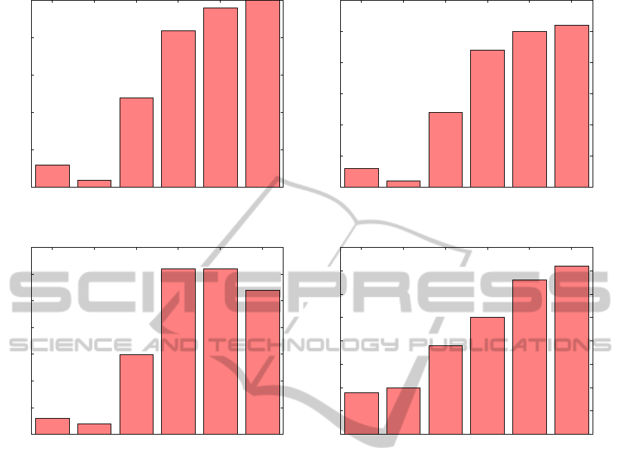
5.7 Comparison
For all the algorithms used for comparison, four dif-
ferent sizes (20, 50, 80, 100) of the recommenda-
tion list were considered. The ordering of the algo-
rithms according to their performances are similar for
all these list sizes. We report the results for the top-50
recommendations.
5.7.1 Amazon Music Dataset
Figure 3(a) and Figure 4(a) compare the Hit Rate
and MRR for Amazon Music dataset. According to
the results, the four algorithms defined in this pa-
per perform better than the algorithms mentioned in
Section 5.4 according to both the evaluation metrics.
Among the algorithms defined in this paper, the sim-
ple baseline method CNT that does not look at the
time information performs the worst. The RECK al-
gorithm that considers the last few purchases of the
target user for expert selection does better than CNT.
Algorithm RECKW that builds upon RECK by us-
ing time weighting on the experts’ purchases achieves
even better Hit Rate for this dataset. The DISCHIST
algorithm that looks at all purchases of all the users
but with discounted importance on the old purchases
achieves the highest Hit Rate.
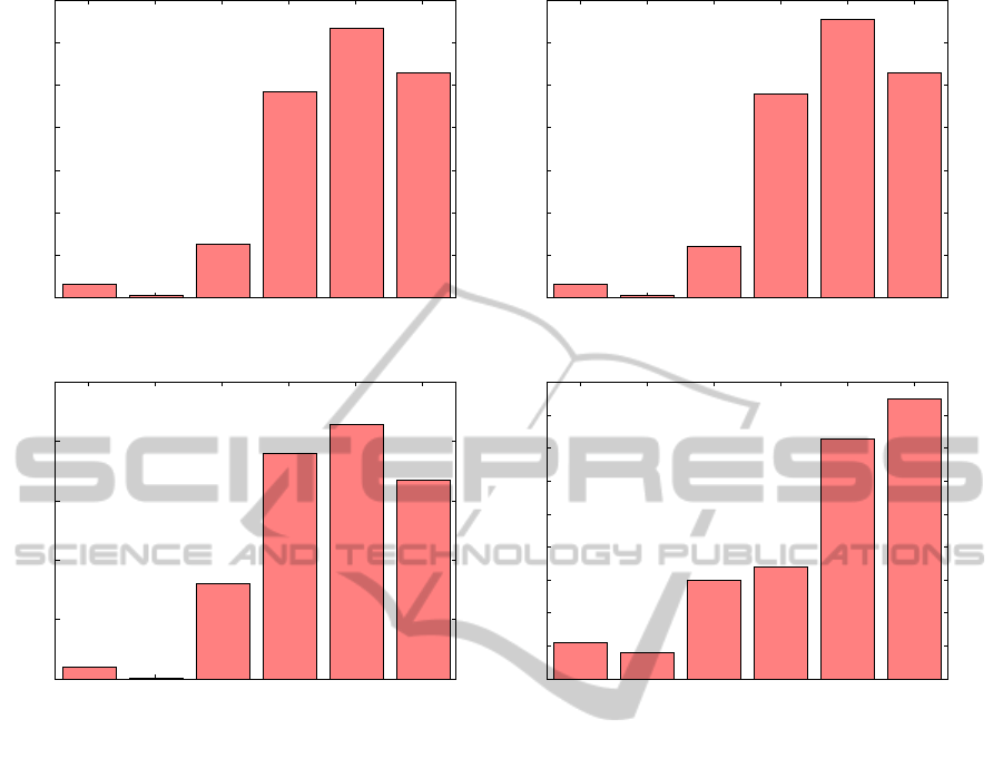
It can be seen from figure 4(a) that RECKW has
maximum MRR, i.e. it is able to put maximum num-
ber of test items at the best (minimum) rank position
among the competitor algorithms. DISCHIST comes
next in terms of MRR. Ordering of the remaining al-
gorithms for this measure is similar to the ordering
obtained for the Hit Rate measure.
5.7.2 Amazon DVD Dataset
The results for this dataset are similar to the results
obtained for the Amazon Music dataset. Hit Rates of
the algorithms are shown in Figure 3(b). DISCHIST
gives the best performance according to this measure
and is closely followed by RECKW.
UserbasedCollaborativeFilteringwithTemporalInformationforPurchaseData
61
0
0.05
0.1
0.15
0.2
0.25
PID WCM CNT RECK RECKW DISCHIST
(a) Hit Rate for Amazon Music dataset
0
0.05
0.1
0.15
0.2
0.25
0.3
PID WCM CNT RECK RECKW DISCHIST
(b) Hit Rate for Amazon DVD dataset
0
0.05
0.1
0.15
0.2
0.25
0.3
0.35
PID WCM CNT RECK RECKW DISCHIST
(c) Hit Rate for Amazon Book dataset
0
0.05
0.1
0.15
0.2
0.25
0.3
0.35
0.4
PID WCM CNT RECK RECKW DISCHIST
(d) Hit Rate for Netflix dataset
Figure 3: Comparison of Hit Rate for different datasets.
Figure 4(b) compares the MRR for all the algo-
rithms. It can be seen from the figure that RECKW
achieves highest MRR. DISCHIST comes second ac-
cording to this metric. It means that ReckW and Dis-
cHist are able to put the test item near the top of the
recommended list for most of the test transactions.
5.7.3 Amazon Book Dataset
Hit Rate and MRR for the Amazon Book dataset are
shown in Figure 3(c) and Figure 4(c) respectively.
These results are somewhat different from the results
obtained for the Amazon Music dataset and Amazon
DVD dataset. Here we see that both RECKW and
RECK perform best according to Hit Rate. For MRR,
RECKW is the best algorithm and is closely followed
by RECK. DISCHIST appears at the third position for
this dataset, for both the metrics.
The results seem to indicate that for Amazon Book
dataset, it might be wise to look at only the recent
purchases of the target user. Looking at the entire
purchase history of the user, even with time weighted
discounted model as suggested in DISCHIST, might
reduce the performance of the recommendation. A
reason behind this might be that users have very fo-
cused interest for book items and this interest shifts
over time. Users purchase books belonging to only
the type(s) that they are currently interested in. As
for music and DVDs, they might have interest in sev-
eral types simultaneously and their recent purchases
are mix of items belonging to all those types.
5.7.4 Netflix Dataset
Experiments on the Amazon datasets showed that
the algorithms that give importance to the time-of-
purchase information achieve better performances.
This observation was corroborated by the results ob-
tained on the Netflix dataset.
Hit Rate comparison for the Netflix dataset is
shown in Figure 3(d). These results are similar to the
results observed for the Amazon Music dataset and
Amazon DVD dataset. DISCHIST performs best ac-
cording to this metric. Comparison of MRR values
KDIR2012-InternationalConferenceonKnowledgeDiscoveryandInformationRetrieval
62
0
0.02
0.04
0.06
0.08
0.1
0.12
0.14
PID WCM CNT RECK RECKW DISCHIST
(a) Mean Reciprocal Rank for Amazon Music dataset
0
0.02
0.04
0.06
0.08
0.1
0.12
0.14
PID WCM CNT RECK RECKW DISCHIST
(b) Mean Reciprocal Rank for Amazon DVD dataset
0
0.05
0.1
0.15
0.2
0.25
PID WCM CNT RECK RECKW DISCHIST
(c) Mean Reciprocal Rank for Amazon Book dataset
0
0.01
0.02
0.03
0.04
0.05
0.06
0.07
0.08
0.09
PID WCM CNT RECK RECKW DISCHIST
(d) Mean Reciprocal Rank for Netflix dataset
Figure 4: Comparison of Mean Reciprocal Rank for different datasets.
is shown in Figure 4(d). For this dataset, DISCHIST
is the best algorithm according to MRR. Performance
of RECKW is also quite good as indicated by the fig-
ure. Performances of PID and WCM algorithms are
much better for this datsaet when compared to their
performances on the other datasets mentioned above.
5.8 Discussions
Overall, DISCHIST and RECW perform the best ac-
cording to the experimental results. We consider
CNT as the baseline for our experiments. Aver-
age Hit Rates of CNT, DISCHIST and RECKW for
the test transactions over all the four datasets are
.148, .288 and .287 respectively. Hence, DISCHIST
and RECKW achieve close to 100% improvement in
Hit Rate over the baseline. Similarly, average MRR
for the three algorithms are .044,.121 and .142 re-
spectively. So, for MRR, RECW and DISCHIST
achieve close to 230% and 175% improvements re-
spectively over the baseline. Both DISCHIST and
RECKW give importance to the recent purchases of
the target user as well as the experts, and hence at-
tempt to address the issues of both user dynamics and
the item dynamics.
Looking at the individual datasets, we see that
for the Amazon Music and DVD datasets and the
Netflix dataset, DISCHIST performs the best accord-
ing to Hit Rate. RECKW and RECK come next in
terms of performance. According to MRR, algo-
rithms RECKW and DISCHIST perform the best. The
trend is little different for the Amazon Book dataset
where RECKW and RECK are better than DISCHIST.
It means that for this dataset, the algorithms should
only consider the most recent purchases of the test
user and use that for expert selection. This may be
due to the fact that users have very focused interest in
a very limited set of categories or sub-categories for
book items. It appears that the size of that interest set
is much smaller for book data, when compared with
the same for Music, DVD or Movie data. Hence giv-
ing importance to purchases made long back, even if
the importance weights for those items are low, act
as distraction for the recommendation algorithms. In
this work, we have used the same parameters to spec-
ify the decay function for all the datasets. However,
UserbasedCollaborativeFilteringwithTemporalInformationforPurchaseData
63

depending on the domain of the items or the selling
trend of the individual items, different parameters can
be used for the decay function for different datasets or
even for individual items.
6 CONCLUSIONS
In this work, we have explored a few time-aware user
based collaborativefiltering algorithms for the recom-
mendation problem. We have analyzed the benefits
of using the time-of-purchase information in both the
phases of expert selection and recommendation gen-
eration. Giving importance to time factor in the ex-
pert selection phase tries to address the problem of the
target user’s interest shift. Giving importance to the
most recent items purchased by the experts attempts
to capture the item dynamics. Experimental results
indicate that recommendationperformancecan be im-
proved by giving more importance to the recent pur-
chases of both the user and the experts.
ACKNOWLEDGEMENTS
The first author is supported by a PhD Fellowship
from Microsoft Research India.
REFERENCES
Campos, P. G., Bellog´ın, A., D´ıez, F., and Chavarriaga, J. E.
(2010). Simple time-biased knn-based recommenda-
tions. In Proceedings of the Workshop on Context-
Aware Movie Recommendation, CAMRa ’10, pages
20–23.
Deshpande, M. and Karypis, G. (2004). Selective markov
models for predicting web page accesses. ACM Trans.
Internet Technol., 4:163–184.
Ding, Y. and Li, X. (2005). Time weight collaborative fil-
tering. In Proceedings of the 14th ACM international
conference on Information and knowledge manage-
ment, CIKM ’05, pages 485–492.
Ding, Y., Li, X., and Orlowska, M. E. (2006). Recency-
based collaborative filtering. In Proceedings of the
17th Australasian Database Conference - Volume 49,
ADC ’06, pages 99–107.
Herlocker, J., Konstan, J. A., and Riedl, J. (2002). An em-
pirical analysis of design choices in neighborhood-
based collaborative filtering algorithms. Inf. Retr.,
5:287–310.
Kawamae, N., Sakano, H., and Yamada, T. (2009). Per-
sonalized recommendation based on the personal in-
novator degree. In Proceedings of the third ACM con-
ference on Recommender systems, RecSys ’09, pages
329–332.
Koren, Y. (2008). Factorization meets the neighborhood:
a multifaceted collaborative filtering model. In Pro-
ceeding of the 14th ACM SIGKDD international con-
ference on Knowledge discovery and data mining,
KDD ’08, pages 426–434.
Koren, Y. (2009). Collaborative filtering with temporal dy-
namics. In Proceedings of the 15th ACM SIGKDD
international conference on Knowledge discovery and
data mining, KDD ’09, pages 447–456.
Lee, T. Q., Park, Y., and Park, Y.-T. (2008). A time-based
approach to effective recommender systems using im-
plicit feedback. Expert Syst. Appl., 34:3055–3062.
Parameswaran, A. G., Koutrika, G., Bercovitz, B., and
Garcia-Molina, H. (2010). Recsplorer: recommen-
dation algorithms based on precedence mining. In
Proceedings of the 2010 international conference on
Management of data, SIGMOD ’10, pages 87–98.
Rendle, S., Freudenthaler, C., and Lars, S.-T. (2010). Fac-
torizing personalized markov chains for next-basket
recommendation. In Proceedings of the 19th inter-
national conference on World wide web, WWW ’10,
pages 811–820.
Rongfei, J., Maozhong, J., and Chao, L. (2010). Using tem-
poral information to improve predictive accuracy of
collaborative filtering algorithms. In Proceedings of
the 2010 12th International Asia-Pacific Web Confer-
ence, APWEB ’10, pages 301–306.
Shani, G., Heckerman, D., and Brafman, R. I. (2005). An
mdp-based recommender system. J. Mach. Learn.
Res., 6:1265–1295.
Zheng, N. and Li, Q. (2011). A recommender system based
on tag and time information for social tagging sys-
tems. Expert Syst. Appl., 38:4575–4587.
KDIR2012-InternationalConferenceonKnowledgeDiscoveryandInformationRetrieval
64
