
Formal Concept Analysis for the Interpretation of Relational
Learning Applied on 3D Protein-binding Sites
Emmanuel Bresso
1,2
, Renaud Grisoni
2
, Marie-Dominique Devignes
1,2,3
,
Amedeo Napoli
1,2,3
and Malika Smail-Tabbone
1,2
1
Université de Lorraine, LORIA, UMR 7503, Vandoeuvre-les-Nancy, F-54506, France
2
Inria, Villers-lès-Nancy, F-54600, France
3
CNRS, LORIA, UMR 7503, Vandoeuvre-les-Nancy, F-54506, France
Keywords: Inductive Logic Programme, Formal Concept Analysis, Knowledge Discovery, 3D Protein Binding Sites.
Abstract: Inductive Logic Programming (ILP) is a powerful learning method which allows an expressive
representation of the data and produces explicit knowledge in the form of a theory, i.e., a set of first-order
logic rules. However, ILP systems suffer from a drawback as they return a single theory based on heuristic
user-choices of various parameters, thus ignoring potentially relevant rules. Accordingly, we propose an
original approach based on Formal Concept Analysis for effective interpretation of reached theories with the
possibility of adding domain knowledge. Our approach is applied to the characterization of three-
dimensional (3D) protein-binding sites which are the protein portions on which interactions with other
proteins take place. In this context, we define a relational and logical representation of 3D patches and
formalize the problem as a concept learning problem using ILP. We report here the results we obtained on a
particular category of protein-binding sites namely phosphorylation sites using ILP followed by FCA-based
interpretation.
1 INTRODUCTION AND
MOTIVATION
Relational or logical learning is currently one of the
most promising research topics in knowledge
discovery, especially for complex application
domains (De Raedt, 2008). Life sciences provide a
wide variety of such applications. In our work we
investigate how relational learning can contribute to
the understanding of protein-protein interactions
which are important for most cellular processes.
Great effort has been put on both experimental and
computational methods to identify or predict
protein-protein interactions. In protein docking,
geometric and steric considerations are used to fit
two protein structures into a bound complex (Smith
et al., 2002). Alternative computational methods
predict bindings between pairs of proteins based
either on their homology with known binding pairs
of proteins or on integrated data from a wide variety
of sources (Aloy and Russel, 2003; Jansen et al.,
2003; Tran et al., 2005). However, despite the large
number of reported computational methods, the
precise understanding of protein-protein
interactions still raises various challenges.
On the one hand, most reported methods for
structure-based prediction of protein-protein
interactions work on a single data table where each
interaction site (or interface) is described by a set of
descriptors or attributes including diverse physico-
chemical properties aggregated on the whole
binding site such as the residue composition,
hydrophobicity, accessible surface area (Jones and
Thornton, 1997; Zhu et al., 2006). However, this
data model prevents from representing individual
properties of the interface components (accessible
surface of a particular residue) or spatial relations
between components (e.g., distance between two
residues). Hence, more expressive languages are
necessary to represent the structural aspect of 3D
interaction sites. Such sites are called hereafter
Protein-Binding Sites (PBS) to make a clear
distinction from ligand-binding sites on protein
surface.
On the other hand, most current methods do not
provide explicit characterization of PBS along with
the prediction model. For instance, methods based
on Support Vector Machines (SVM) act as black-
111
Bresso E., Grisoni R., Devignes M., Napoli A. and Smaïl-Tabbone M..
Formal Concept Analysis for the Interpretation of Relational Learning Applied on 3D Protein-binding Sites.
DOI: 10.5220/0004149901110120
In Proceedings of the International Conference on Knowledge Discovery and Information Retrieval (KDIR-2012), pages 111-120
ISBN: 978-989-8565-29-7
Copyright
c
2012 SCITEPRESS (Science and Technology Publications, Lda.)

boxes returning outputs with respect to inputs
without explanation (Zhu et al., 2006). Explicit
characterization of PBS would obviously provide
good insights of the underlying biological
phenomena. In this context our aim is to exploit the
growing set of available protein 3D structures for
characterizing PBS and go beyond the limitations of
the most current approaches qualified as black-box
and single-table. To achieve this objective, we
propose to apply an ILP (Inductive Logic
Programming) learning method on the descriptions
of protein 3D patches in order to induce a general
definition of the PBS concept. Our approach
includes a relational representation of protein 3D
patches corresponding to positive or negative
examples of PBS.
Inductive Logic Programming (ILP) allows to
learn a concept definition from observations, i.e., a
set of positive examples (E+) and a set of negative
examples (E-), and background knowledge (B)
(Muggleton, 1991). Given E+, E-, and B the goal of
ILP is to induce a set of rules or a theory T that is
consistent (TB covers or explains each positive
example in E+), and complete (TB does not cover
or contradicts any negative example in E-).
In most ILP systems both B and T are
represented as definite clauses (or prolog programs)
in First-Order Logic (FOL), i.e., a disjunction of
literals with one positive literal. A rule has the form
"head:- body" and is interpreted as: if the conditions
in the body are true then the head is true as a logical
consequence. The background knowledge B
includes (i) the relational description of the
examples using a set of relevant n-ary predicates
and (ii) a priori domain knowledge, i.e., a set of
rules and facts which do not refer to any example
but express what is known about the elements
which describe the examples. The theory T is a set
of rules which cover as many of the positive
examples as possible and the fewest negative
examples. The head of each rule is the concept to
characterize whereas the body contains the induced
description of the concept (generalization of
examples). The rule search is performed in a clause
space where the clause subsumption allows building
generalizations or specializations of the clauses
(Muggleton and De Raedt, 1994). As the clause
space is too large to be exhaustively explored,
heuristic mechanisms exist to reduce its size and
make the induction process feasible. These
mechanisms allow the user to define which kind of
rules(s) he wants to get. These learning biases are
defined by setting some parameters that influence
the search strategy and lead to different theories.
Consequently, albeit ILP systems have important
properties that make them good candidates for
knowledge discovery tasks in complex domains,
they have a major shortcoming which may impede
their usability: a single theory based on heuristics is
returned, thus ignoring many clauses that may be
relevant for the domain expert (Page and Srinivasan
2003). This may partly explain the low impact of
logical learning noticed by King (2011).
Consequently, we propose in this paper an original
approach to complement the ILP-based knowledge
discovery thanks to classification-based
interpretation of different theories. A binary table is
built according to the covering relation between
examples and rules. Formal Concept Analysis
(FCA, Ganter and Wille, 1999) is used to identify in
the table formal concepts grouping examples
covered by the same rules.
For a first validation of our approach, we chose
a specific group of PBS, the phosphorylation sites.
Indeed, phosphorylation is an important biological
process and phosphorylation sites are exhaustively
listed in a unique data source (Diella et al., 2008).
The rest of the paper is organized as follows.
Section 2 introduces the knowledge discovery
problem and the ILP program we used along with
the different experimental settings. Section 3
describes our proposal for theory interpretation
using FCA and domain knowledge. Section 4
summarizes the results obtained with our
application on PBS. We discuss our results and
describe related work in Section 5.
2 ILP FOR CHARACTERISING
3D PROTEIN-BINDING SITES
2.1 The Data Representation
Language
Protein 3D Patch Definition: Protein surface
patches were first introduced by Jones and Thornton
(1997) who defined a surface patch as a central
surface accessible residue (amino acid) along with
the nearest surface accessible neighbours. For our
part, we define a protein 3D patch as a spherical
fragment of a protein 3D structure centred on a
residue of the protein, the central core residue
(Guharoy and Chakrabarti, 2005). A 3D patch has a
radius r corresponding to the sphere radius and the
residues composing the patch are those having an
atom whose distance to the central residue does not
exceed r. The RCSB PDB database (www.pdb.org)
stores the resolved 3D structures of proteins
KDIR2012-InternationalConferenceonKnowledgeDiscoveryandInformationRetrieval
112

(Berman et al., 2000).
Protein 3D Patch descriptors: We propose to
describe a 3D patch at two levels: (i) the patch is
characterized as a whole by a set of global
descriptors such as patch solvent accessible surface
area (ASA), the number of carbon atoms occurring
in the patch, and the number of residues in the
patch; (ii) the patch composition and structure are
characterized by a set of descriptors describing
secondary and tertiary structure information on the
patch residues. At the latter level, each residue of
the patch is described by its name and its relative
position in the primary sequence of the protein with
respect to the central residue of the patch. The ASA
value of each residue is used as a local descriptor of
the residue in the patch. Two descriptors indicate if
a given residue is on a helix, respectively on a
sheet. Finally, one descriptor represents the spatial
distance between each patch residue and the central
residue. This distance information may play an
important role in the interaction building. Figure 1
shows an example of a protein 3D patch. The
variety of relationships between the elements of a
patch clearly requires a relational or logical
representation language as a feature-based language
could only represent the global descriptors of the
patches.
Figure 1: Visualization of a protein (PDB ID: 1opk) 3D
patch using the VMD program (Humphrey et al., 1996).
The central residue of the patch is represented in red. The
patch surface accessible to the solvent is represented in
blue.
Characterization of 3D PBS as a relational
learning problem: Our objective is to learn with
ILP a definition of the Protein-Binding Site concept
given relational descriptions of positive and
negative examples of this concept.
We define a set of first-order predicates relevant
for the ILP problem (Table 1). The unary predicate
"pbs" is the concept to characterize and has a 3D
patch identifier as argument. Several binary
predicates represent the global descriptors of the
patch such as the predicates "p_asa" and "p_c"
which correspond respectively to the ASA value of
a patch and the number of carbon atoms. A set of
ternary and 4-ary predicates represent the structural
descriptors of the 3D patches. One 4-ary predicate
is "p_r_distance" which represents the distance
value of a patch residue from the central residue.
One ternary predicate is "p_r_helix" which
expresses that a patch residue belongs to a helix. A
supplementary ternary predicate is "p_r_surface"
which is derived from the "p_r_asa" predicate.
Finally, a prolog rule allows to infer that a residue is
on the patch surface if its ASA value is greater than
the threshold 10Ų:
p_r_surface (pid,res,pos) :‐ p_r_asa (pid,res,pos,v),
greater_than(v,10).
As mentioned before, ILP allows to use domain
knowledge during the induction process. In our
case, there is a consensus to classify the different
residues in several classes reflecting shared
physico-chemical properties which may play a role
in protein-protein interfaces (Jones and Thornton,
1997). Hence, we choose to use two classifications
as a priori domain knowledge (Table 2).
Consequently, we define a unary predicate for each
residue class (e.g., acidic, basic) whose
interpretation is defined according to the class
membership (e.g., acidic(asp),basic(arg)).
Table 1: First order-logic predicates to describe protein
3D patches.
Predicate Interpretation
pbs(pid)
The patch identified by pid is a protein-
binding site
p_asa(pid,v)
v is the solvent accessible surface value
of the pid patch
p_c(pid,n),p_o(pid,n),
p_n(pid,n),p_s(pid,n)
n is the number of
carbon/oxygen/nitrogen/sulphur atoms in
the pid patch
p_r(pid,res,pos)
res is the name of the residue at relative
position pos in the pid patch
p_r_asa(pid,res,pos,v)
v is the ASA value of the residue named
res at the relative position pos (in the
primary sequence) in the pid patch
p_r_distance
(pid,res,pos,v)
v is the spatial distance between the
residue (res, pos) and the central residue
in the pid patch
p_r_helix(pid,res,pos),
p_r_sheet(pid,res,pos)
the residue (res, pos) is on a helix/sheet in
the pid patch
FormalConceptAnalysisfortheInterpretationofRelationalLearningAppliedon3DProtein-bindingSites
113

Table 2: Physico-chemical classes of residues defined in
(Yu et al., 2006) and (Dubchak et al., 1999).
Class Name Residues in the Class
acidic asp, glu
basic arg., hais, lys
aromatic phe, trp, yr
amide asn, gln
small hydroxyl ser, thr
sulphur containing cys, met
aliphatic1 ala, gly, pro
aliphatic2 ile, leu, val
aliphatic ala, gly, pro, ile, leu, val
small gly,ala,ser,cys,thr,pro,asp
medium asn, val, glu, gln, ile, leu
large met, his, lys, phe, arg, tyr, trp
low polarizability gly, ala, ser, asp, thr
medium polarizability cys, pro, asn, val, glu, gln, ile, leu
high polarizability lys, met, his, phe, arg, tyr, trp
hydrophobic cys, val, leu, ile, met, phe, trp
To sum up, the global and structural descriptors are
computed for a set of 3D patches and represented
with respect to the defined FOL predicates, forming
a learning set. A ILP program can then be used to
learn FOL rules characterizing or covering subsets
of positive patches.
2.2 The ILP Program and Its
Parameters
The experiments reported in this paper were
conducted with the Aleph program whose basic
algorithm is described in four steps (Srinivasan,
2007):
1. Select one positive example to be generalized,
called seed example. If none exists, stop.
2. Construct the most specific clause that entails
the example selected, and is compliant with the
language restrictions provided. This is usually a
definite clause with many literals, and is called the
"bottom clause".
3. Find a clause more general than the bottom
clause. This is done by searching for some subset of
the literals in the bottom clause that has the best
evaluation score.
4. The clause with the best score is added as a
rule to the current theory, and all examples made
redundant are removed. Return to Step 1.
Many parameters can be set for tuning some
aspect of the theory construction with Aleph. For
instance, the rule evaluation function can be chosen
and the default one is based on the difference
between the number of covered positive examples
and the number of covered negative examples. The
noise parameter is the maximum negative examples
that an acceptable rule may cover (default value is
0). This parameter can be set to higher values in
case of noisy data (in our study, one is never sure
that a negative PBS is a true one unless
experimental evidence is provided). The min-pos
parameter is the minimal number of positive
examples that a rule must cover (default value is 1).
Aleph also requires other learning biases to be
defined as (i) a set of determinations defines the
predicate to learn and the predicates which can
appear in the rules; (ii) a set of modes defines the
types of predicate arguments and the way they can
be chained in a rule.
As the above algorithm suggests, Aleph iterates
on the positive examples of the learning set for
building the most specific clause of a chosen seed
example which is compliant with the defined bias
and covers the maximum number of positive
examples and the minimum number of negative
ones. When finding the best rule, the examples
covered by the best rule may be removed or not
from the seed set and/or from the learning set (used
for the rule evaluation). Hence with regard to this
removal step, a induce-type parameter defines three
ways of theory construction, (i) induce (covered
examples are removed from both the seed set and
the learning set), (ii) induce-cover (covered
examples are removed from the seed set and not
from the learning set), and (iii) induce-max
(covered examples are removed neither from the
seed set nor the learning set). Consequently, both
induce and induce-cover are sensitive to the order in
which the seed examples are presented contrasting
with induce-max (each example is generalized).
Both induce-cover and induce-max produce rules
with more overlap than induce.
3 FCA-BASED
INTERPRETATION OF A
THEORY
Different theories are reached by the ILP program
depending on the values of the program parameters
set by the user in a heuristic way. It is then
important to allow the domain expert to explore
each theory. Each theory is globally characterized
by the learning set coverage, i.e., the proportion of
positive examples that are covered by at least one
rule of the theory (theory coverage). Another global
criterion is the coverage of the best rule.
Furthermore, we propose a FCA-based analysis of
the ILP learning results including or not domain
knowledge to help the expert in the interpretation
task. This can possibly lead to one or more
KDIR2012-InternationalConferenceonKnowledgeDiscoveryandInformationRetrieval
114

preferred theories.
3.1 Formal Concept Analysis (FCA)
The framework of FCA is fully detailed in (Ganter
and Wille, 1999). FCA starts with a formal context
(G,M,I) where G denotes a set of objects, M a set of
attributes, and I G
X M a binary relation between
G and M. The statement (g,m) I is interpreted as
"the object g has attribute m" (also noted gIm). Two
operators (.)' define a Galois connection between
the powersets (2
G
, ) and (2
M
, ), with A G and
B M:
A' = {m
M |
g
A : gIm} and
B' = {g
G |
m
B : gIm}
For A G, B M, a pair (A,B), such that A' = B
and B' = A, is called a formal concept. In (A,B), the
set A is called the extent and the set B the intent of
the concept (A,B). Formal concepts are partially
ordered by the concept subsumption:
(A1, B1) ≤ (A2,B2) A1 A2 B2 B1.
With respect to this partial order, the set of all
formal concepts forms a full lattice called the
concept lattice of (G,M,I). The FCA
implementation used in our experiments was the
one of the Coron data mining platform (Szathmary,
2006)
3.2 FCA-based Analysis of an ILP
Theory
A first interpretation of a theory is defined on the
concept lattice issued from FCA applied on the
binary patch-rule matrix describing the coverage of
positive examples by the rules (only the body part
of the rules is necessary since the head is the same
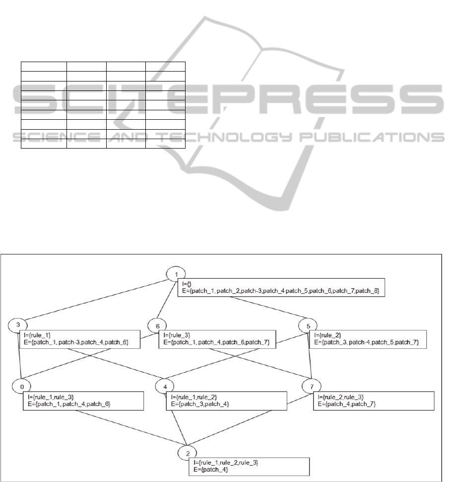
for all rules). Table 3 shows an example of a formal
context with 8 patches and 3 rules. In our case, a
formal concept gathers a subgroup of 3D patches
which are covered by the same set of rules. Figure 2
shows the concept lattice obtained from the context
presented in Table 3. The concept lattice forms a
good artefact for browsing the ILP results allowing
the expert to move from a set of patches covered by
one rule to more specific concepts containing
subsets of the patches covered by two rules, three
rules and so on. Indeed, it is relevant to count for
each theory, the number of concepts of more than
two rules (multiple-rule concepts) and having a
significant extent size (number of patches).
Furthermore, multiple-rule concepts can be
examined by the domain expert to check whether
any concept intent (rule conjunction) provides a
relevant description of the corresponding patch
subgroup.
A second interpretation of a theory is defined on
the results of FCA applied to the patch-rule
covering matrix enriched with supplementary
domain properties of the examples that were not
used in the learning process. This allows the expert
to analyze how the theory rules are related to known
properties of the examples. More precisely,
interesting concepts to look at are concepts whose
intent includes specific properties along with rules
and whose extent has a significant size. These
formal concepts gather 3D patches sharing domain
property(ies) and being covered by the same rule(s).
Involved rule(s) will be said to be associated with
the domain property(ies).
4 RESULTS
As a first validation, we apply our approach to a
particular category of protein-binding sites, i.e.,
phosphorylation sites. We first present the learning
set we established (Section 4.1) and the results of
the FCA-based interpretation of 18 theories we have
achieved using the Aleph program (Section 4.2).
4.1 The Learning Dataset of the Case
Study
Phosphorylation is a reversible post-translation
modification of a protein due to a kinase adding a
phosphate group to a serine, threonine, or a tyrosine
residue
(so called phosphorylated residue). A set of
experimentally verified eukaryotic Phosphorylation
Sites (PS) is available in the Phospho.ELM
database (Diella et al., 2008). In this study, we build
a learning set including all known phosphorylation
sites irrespective of the phosphorylating kinase and
the phosphorylated residue. This contrasts with the
systems which perform the prediction of residue-
specific or kinase-specific phosphorylation sites
(Wong et al., 2007; Durek et al., 2009). The PS
concern about 5 976 distinct proteins among which
only 286 have exploitable 3D structures. The PS
relative to those proteins divide into 231 serine
sites, 90 threonine sites, and 193 tyrosine sites. For
each PS we extract one positive 3D patch from the
PDB best-resolution 3D structure of the
corresponding protein. This patch is centered on the
phosphorylated residue (serine, threonine, or
tyrosine). As for negative examples, given a protein
structure for which PS are known, biologists are
able to identify with reasonable confidence 3D
FormalConceptAnalysisfortheInterpretationofRelationalLearningAppliedon3DProtein-bindingSites
115
patches corresponding to negative PS. Thus, a
negative 3D patch is built for each
serine/threonine/tyrosine residue which is not
known as a phosphorylable residue and whose
minimal spatial distance to a phosphorylable
residue is reasonably high (greater than 10Å in our
experiments). The total number of found negative
examples is 687 representing 57% of the learning
dataset. The proposed descriptors for protein
patches are computed on the basis of the 3D
coordinates of the patch atoms extracted from the
PDB structures. The numeric descriptor values were
discretized by equal-frequency binning.
Table 3: Formal context example
rule_1 rule_2 rule_3
patch_1 x x
patch_2
patch_3 x x
patch_4 x x x
patch_5 x
patch_6 x x
patch_7 x x
patch_8
Our objective is the 3D PBS characterization
instead of their prediction especially as there exist
for the phosphorylation case sequence-based
prediction programs which exhibit good
performances (Wong et al., 2007). Besides, the
amount of available protein 3D structures is fairly
smaller than the available protein sequences making
it difficult to reach the prediction accuracy of those
programs. Nevertheless, the prediction accuracy of
a ILP theory (defined as the number of true
positives plus true negatives over the total number
of examples) is interesting to consider for building
the learning set and comparing different theories.
Hence theory prediction accuracy was computed by
a tenfold cross-validation test for variable negative
example percentages in the learning set (induce type
and min-pos are set to induce-cover and 13). The
results are given in Table 4 and confirm that the
prediction accuracy continuously increases with the
percentage of negative example. It is thus relevant
to use the whole set of found negative 3D patches
(i.e., 57% negative examples versus 43% positive
examples).
4.2 FCA-based Interpretation of ILP
Theories
In our experiments, we consider three parameters
which alter the way the rule search is seeded and
the rules are selected in the Aleph program: induce-
type (induce, induce-cover, induce-max), min-pos
(from 8 to 12), and noise (0 or 1). The rest of the
parameters were set to the default value. In order to
reduce the number of theories to interpret, we used
as theory ranking criterion the prediction accuracy
value (tenfold cross validated). We selected the 18
theories having a prediction value greater than 60%.
Actually the accuracy values vary from 54 to 63%.
Figure 2: The concept lattice obtained by FCA from Table 3. Each numbered concept has an intent (I) and an extent (E).
The edges correspond to subsumption relationships.
KDIR2012-InternationalConferenceonKnowledgeDiscoveryandInformationRetrieval
116

As mentioned before the relatively weak values of
prediction accuracy can be explained by the small
size of the training set due to the small number of
currently available 3D structures and its
heterogeneity with respect to the phosphorylated
residue and the phosphorylating kinase. The global
criteria and the quantitative results of the FCA-based
interpretation of the 18 selected theories are reported
in Table 5. We notice that, the parameters have a
combined effect on the theory size, the theory
coverage and the best rule coverage as well as on the
concept lattice composition. The most obvious trend
is the continuous decrease of theory size, theory
coverage and the number of multiple-rule concepts
when increasing min-pos for a given induce-type
and noise value. This makes the choice of an optimal
configuration difficult because some trade-off must
be found between these criteria. For instance, a
small size is expected for a valuable theory but this
should not be at the expense of its coverage.
Table 4: Prediction accuracy values (tenfold cross
validated) obtained when varying the negative example
percentage in the learning set.
Percentage of
negative examples
Noise
parameter
Prediction accuracy
35 0 52
35 1 54
40 0 54
40 1 55
45 0 54
45 1 55
50 0 55
50 1 57
55 0 58
55 1 58
57 0 59
57 1 61
Table 5: Quantitative results of the FCA applied on the
patch-rule covering matrices for the 18 selected theories.
Theory
parameters
(induce-type/
min-pos)
Theory size
/ best rule
coverage
Theory
coverage (%)
# multiple-rule
concepts/ best
concept extent
size
noise=0
induce-cover/9 64/ 15 56 106/ 9
induce-cover/10 37/ 16 39 71/ 14
induce- max /9 64/ 15 56 106/ 9
induce-max/10 39/ 16 39 88/ 14
noise=1
induce/8 26/ 17 48 8/ 3
induce/9 19/ 17 39 5/ 3
induce /10 14/ 16 32 3/ 3
induce /11 10/ 15 24 0/0
induce-cover/10 85/ 18 73 215/ 13
induce-cover/11 58/ 18 61 144/ 16
induce-cover/12 38/ 18 48 91/ 13
induce-cover/13 20/ 18 30 50/ 13
induce-cover/14 15/ 18 23 31/ 16
induce-max/10 101/ 18 73 386/ 16
induce-max/11 69/ 18 61 254/ 16
induce-max/12 43/ 18 48 136/ 16
induce-max/13 24/ 18 30 80/ 16
induce-max/14 15/ 18 23 31/ 16
To illustrate the effect of the induce-type
parameter on the clause search, the theory reached
with the induce/10/1 configuration is provided
(Appendix). One rule found in a different
configuration (induce-max/10/1) and missing in the
previous theory is the following:
pbs(A) :‐ p_r_helix(A,B,3), high_polarizability(B),
p_r(A,pro,1).
This rule covers 17 positive examples but is not
retrieved when switching the induce-type parameter
from induce-max to induce.
To illustrate the browsing process in the concept
lattice, we examined multiple-rule concepts from the
18 lattices. For instance, the theory with induce-
max/12/1 produces a formal concept of 14 patches
sharing the two following rules:
pbs(A):‐p_r_surface(A,B,0),p_r_helix(A,C,21),
p_r_helix(A,D,28).
pbs(A):‐p_r_surface(A,B,0),p_r_helix(A,C,17),
p_r_helix(A,D,28).
When browsing up the lattice, we find a subgroup
composed of 11 patches which share the two
previous rules besides the following third one:
pbs(A):‐p_r_surface(A,B,0),p_r_helix(A,C,20),
p_r_helix(A,D,28).
Hence, this subgroup of 11 patches is better
characterized by the conjunction of the three rule
bodies (after variable renaming and removal of
redundant literals):
p_r_surface(A,B,0),p_r_helix(A,C,21),p_r_helix(A,D,28),
p_r_helix(A,E,17),p_r_helix(A,F,20).
In more general terms, selecting formal concepts
with multiple rules constitutes an interesting way to
achieve longer rules than in the theory issued by
Aleph. Indeed, the compression heuristic used
during the clause search leads most ILP programs to
favor shorter clauses to longer ones. Finn et al.,
(1998) proposed a solution to this drawback suitable
to the pharmacophore search case.
An additional way to explore the concept lattices
is to count how many multiple-rule concepts are
enriched in specific patches with respect to the
phosphorylated residue (serine or threonine versus
tyrosine). Over the 18 analysed lattices we observed
that more than 75% of the multiple-rule concepts are
either tyrosine specific or serine-or-threonine
specific. This provides the expert with relevant
descriptions for each type of phosphorylation sites as
well as descriptions common to both types.
FormalConceptAnalysisfortheInterpretationofRelationalLearningAppliedon3DProtein-bindingSites
117

4.3 FCA-based Interpretation of ILP
Theories including Domain
Knowledge
We applied FCA on the patch-rule table enriched
with supplementary domain properties of the
examples not used in the learning process, namely
the phosphorylating kinase and the functional
domain on which the 3D patch is located (Punta et
al., 2012). ILP produces a set of rules covering 3D
patches and the interpretation procedure we propose
here helps the expert to analyze how the rules are
related to known properties of the examples. About
50 kinases phosphorylate more than 2 patches of the
learning set whereas 40 Pfam domains are associated
to more than 2 patches. The patch-rule table is thus
updated with those kinases and functional domains
as supplementary properties of the patches. Some
formal concepts of the resulting lattice include at
least one rule along with a kinase (respectively a
Pfam domain) and whose extent contains more than
1/3 of the patches associated to the kinase
(respectively the Pfam domain). The rules involved
in such concepts can be examined by the expert in
order to check their consistency with previous
knowledge and whether they reveal novel relevant
knowledge units regarding the kinase (respectively
Pfam domain) concerned. For example the following
rule was found associated with PKB kinases in
concepts grouping the majority of 3D patches
phosphorylated by this type of kinases:
pbs(A):‐p_r_helix(A,B,‐4),p_r_helix(A,arg,‐3),
p_r_helix(A,ser,0).
In this rule the expert recognizes in particular the
fact that an arginine residue is present at position -3
which is a well established observation for PKB
kinases (Obata et al., 2000). More precisely the
second literal expresses that the arginine residue at -
3 position should be on a helix, which reveals to be
interesting for characterizing those 3D patches.
Quantitative analysis of domain-knowledge FCA
was performed in order to help the expert assessing
the relative relevance of a theory with respect to
another one. To this aim, the number of kinases
(respectively Pfam domains) appearing at least once
in a concept with an extent containing at least 1/3 of
the concerned patches was computed for each of the
18 theories selected in this study. The results are
presented in Table 6. Interestingly, it appears that, in
particular with induce-max, the number of kinases
does not continuously decrease with increasing
values of the min-pos parameter. This contrasts with
the continuous decrease of the theory coverage and
size (Table 5). Thus even at low coverage values, the
theory rules still exhibit descriptive ability correlated
with domain knowledge. One can notice that such
low-coverage theories would be discarded if the
objective was prediction instead of characterization.
Table 6: Number of kinases (respectively Pfam domains)
appearing in concepts whose extent contains more than 1/3
of the patches associated to the kinase (respectively Pfam
domain).
Theory parameters (induce-
type/ min-pos)
Kinase
number
Pfam domain
number
noise=0
induce-cover/9 10 10
induce-cover/10 6 8
induce-max /9 10 9
induce-max/10 6 10
noise=1
induce/8 8 8
induce/9 9 9
induce /10 8 8
induce /11 4 6
induce-cover/10
12 11
induce-cover/11 7 10
induce-cover/12 7 7
induce-cover/13 8 4
induce-cover/14 8 2
induce-max/10
12 11
induce-max/11 11 7
induce-max/12 7 7
induce-max/13 8 4
induce-max/14 10 3
5 DISCUSSION
ILP has been successfully applied to various areas
including bioinformatics (Page and Craven, 2003).
Turcotte et al. (2001) used ILP for predicting protein
3D structures. Each protein domain is described by
global features (e.g., length, number of helices),
adjacency relationships between two consecutive 2D
structure elements, and some local properties of the
2D structure elements (e.g., length, presence of some
residue). Another ILP application aimed at
pharmacophore design for virtual screening purposes
(Finn et al., 1998). A pharmacophore is defined as
an abstract 3D structure of a molecule that interacts
with a protein target. In this case, pairwise distances
between atoms or atom groups (e.g., hydrogen
donors) of a set of interacting (respectively not
interacting) molecules with a specific target are
considered for learning. More recently, 3D
information on molecules was exploited for
searching structurally diverse molecules (drugs)
which share a biological activity (Tsunoyama et al.,
2008). The considered 3D descriptors are the spatial
KDIR2012-InternationalConferenceonKnowledgeDiscoveryandInformationRetrieval
118

distances between the atoms composing each active
(respectively inactive) molecule of the learning set.
Finally, ILP was applied on genomic annotations of
proteins coming from public databases (e.g., Pfam,
InterPro, PROSITE) in order to predict protein-
protein interactions for one specific species (Tran et
al., 2005).
To the best of our knowledge, our study is one of
the firsts which characterize 3D protein-binding sites
using ILP. This forms a natural follow-up of
previous applications of ILP focusing on the
prediction of protein 3D structure, as nowadays
protein 3D structures become increasingly available.
As for post-ILP analysis, our approach is
innovative and represents a step forward in the
interpretation of ILP results in the frame of a
knowledge discovery process. Indeed, it offers the
expert an effective assistance when exploring the
learning results including confrontation with domain
knowledge. By facilitating theory interpretation, our
approach puts the tricky problem of heuristic
parameters selection into perspective. It allows to
take benefit from more than one theory. Otherwise,
upstream investigation into the effect of numerous
parameters on discriminative selection criteria is
required as reported in (Turcotte et al., 2001).
We are convinced that our approach can be
adapted to other learning problems. Using FCA
makes it possible to discover higher-level
knowledge units by extracting from the formal
concepts first-order logic association rules between
the ILP rule bodies (Pasquier et al., 1999). Another
perspective of this study concerns the scaling up of
ILP programs. Theories can be produced on distinct
descriptors subsets corresponding to distinct views
on the examples. FCA-based joint interpretation of
the resulting theories can then enable the discovery
of rules involving descriptors from the distinct
subsets.
REFERENCES
Aloy, P., Russell, R., 2003. InterPreTS: Protein Interaction
Prediction through Tertiary Structure. Bioinformatics
Applications Note, 19 (1): 161-162.
Berman, H. M., Westbrook, J., Feng, Z., Gilliland, G.,
Bhat, T. N., Weissig, H., Shindyalov, I. N., Bourne, P.
E., 2000. The Protein Data Bank. Nucleic Acids
Research, 28: 235-242.
De Raedt L., 2008. Logical and Relational Learning.
Springer.
Diella, F., Gould, C. M., Chica, C., Via, A., Gibson, T. J.,
2008. Phospho.ELM: a database of phosphorylation
sites – update 2008. Nucleic Acids Res., 36 (Database
issue): D240-4.
Dubchak, I., Muchnik, I., Mayor, C., Dralyuk, I., Kim, S-
H., 1999. Recognition of a protein fold in the context
of the SCOP classification. Proteins: Structure,
Function, and Genetics, 35(4): 401-407.
Durek, P., Schudoma, C., Weckwerth, W., Selbig, J.,
Walther, D., 2009. Detection and characterization of
3D-signature phosphorylation site motifs and their
contribution towards improved phosphorylation site
prediction in proteins. BMC Bioinformatics., 10: 117.
Finn, P., Muggleton, S., Page, D., Srinivasan, A., 1998.
Pharmacophore Discovery Using the Inductive Logic
Programming System PROGOL. Machine Learning,
30(2-3):241-273.
Ganter, B. and Wille, R., 1999. Formal concept analysis:
Mathematical foundations. Springer, Heidelberg,
Germany: Springer.
Guharoy, M., Chakrabarti, P., 2005. Conservation and
relative importance of residues across protein-protein
interfaces. PNAS, 102(43):15447-15452.
Humphrey, W., Dalke, A., Schulten, K., 1996. VMD-
Visual Molecular Dynamics. J. Molec. Graphics, 14:
33-38.
Jansen, R., Yu, H., Greenbaum, D., Kluger, Y., Krogan,
N. J., Chung, S., Emili, A., Snyder, M., Greenblatt, J.
F., Gerstein, M., 2003. A Bayesian networks approach
for predicting protein-protein interactions from
genomic data. Science, 302(5644): 449-53.
Jones, S., Thornton, J., 1997. Analysis of protein-protein
interaction sites using surface patches. J. Mol. Biol.,
272: 121-32.
King, R., 2011. Logic, Automation, and the Future of
Biology. Proceedings of the Spring School on
Modelling Complex Biological Systems, Sophia-
Antipolis, France.
Muggleton, S., 1991. Inductive Logic Programming. New
Generation Computing, 8(4): 295-318.
Muggleton, S., and De Raedt, L., 1994. Inductive Logic
Programming: Theory And Methods. Journal of Logic
Programming, 19/20: 629-679.
Obata, T., Yaffe, M. B., Leparc, G. G., Piro, E. T.,
Maegawa, H., Kashiwagi, A., Kikkawa, R., Cantley L.
C., 2000. Peptide and protein library screening defines
optimal substrate motifs for AKT/PKB. J. Biol. Chem.
275, 36108-36115.
Page, D., Craven, M., 2003. Biological applications of
multi-relational data mining. SIGKDD Explorations,
5(1): 69-79.
Page, D., Srinivasan, A., 2003. ILP: A Short Look Back
and a Longer Look Forward. Journal of Machine
Learning Research 4: 415-430.
Pasquier, N., Bastide, Y., Taouil, R., Lakhal, L., 1999.
Efficient mining of association rules using closed
itemset lattices.
Journal of Information Systems, 24(1),
25-46.
Punta, M. et al., 2012. The Pfam protein families database.
Nucleic Acids Research, 40 (Database Issue): D290-
D301.
Smith, G., Sternberg, M., 2002. Prediction of protein-
protein interactions by docking methods. Current
Opinion in Structural Biology, 12(1):28-35.
FormalConceptAnalysisfortheInterpretationofRelationalLearningAppliedon3DProtein-bindingSites
119

Srinivasan, A., 2007. The Aleph Manual. Available at
http://www.comlab.ox.ac.uk/oucl/research/areas/machl
earn/Aleph/.
Szathmary, L., 2006. Symbolic Data Mining Methods with
the Coron Platform. PhD Thesis in Computer Science,
Univ. Henri Poincaré – Nancy 1, France.
Tran, T., Satou, K., Ho, T., 2005. Using Inductive Logic
Programming for Predicting Protein-Protein
Interactions from Multiple Genomic Data. In:
Knowledge Discovery in Databases: PKDD 2005;
Lecture Notes in Computer Science Volume 3721;
Springer Berlin / Heidelberg.
Tsunoyama, K., Ata Amini, A., Sternberg, M., Muggleton,
S., 2008. Scaffold Hopping in Drug Discovery Using
Inductive Logic Programming. Journal of Chemical
Information and Modeling, 48(5):949-957.
Turcotte, M., Muggleton, S., Sternberg, M., 2001.
Automated discovery of structural signatures of
protein fold and function. Journal of Molecular
Biology, 306(3):591-605.
Wong, Yh. et al., 2007. Kinasephos 2.0: A Web Server
For Identifying Protein Kinase-Specific
Phosphorylation Sites Based on Sequences and
Coupling Patterns. Nucleic Acids Res., 35 (Web Server
issue): W588–W594.
Yu, C. S., Chen, Y. C., Lu, C. H., Hwang, J. K., 2006.
Prediction of protein subcellular localization. Proteins,
64: 643-51.
Zhu, H., Domingues, F. S., Sommer, I., Lengauer, T.,
2006. NOXclass: prediction of protein-protein
interaction types. BMC Bioinformatics, 7: 27.
APPENDIX
Rule bodies of the theory induce/10/1. Number of
covered positive/negative examples are given
between square brackets.
p_o(A,29‐inf),p_r_distance(A,B,‐2,6‐8),
p_r_distance(A,C,‐1,0‐6),aliphatic(C).[16,1]
p_r_surface(A,B,0),p_r_helix(A,C,21),
high_polarizability(C).[16,1]
p_r_surface(A,ser,0),p_r(A,pro,1),p_r_distance(A,B,‐2,0‐
6),p_r_distance(A,C,2,0‐6).[15,1]
p_r_helix(A,B,4),p_r_distance(A,C,6,8‐10),p_c(A,105‐inf).
[15,0]
p_r_helix(A,ser,0),p_r(A,r,‐3),p_r_distance(A,B,1,0‐6),
medium_polarizability(B).[15,0]
p_r(A,pro,1),p_r_distance(A,B,‐3,8‐10),
p_r_distance(A,C,‐1,0‐6),medium_polarizability(C).
[15,1]
p_r_helix(A,B,‐2),p_r_distance(A,C,7,10‐11),aliphatic(C).
[14,1]
p_n(A,22‐26),
p_c(A,63‐75).[14,1]
p_r(A,val,‐1),p_r_distance(A,B,‐4,0‐6),
p_r_distance(A,C,8,0‐6).[14,1]
p_r_distance(A,B,‐3,10‐11),p_res(A,46‐inf).[13,1]
p_r_helix(A,B,13),small(B),p_r_helix(A,C,17).[13,1]
p_r(A,arg,‐2),p_r_distance(A,B,‐1,0‐6),basic(B).[13,1]
p_r_distance(A,B,2,6‐8),p_r_distance(A,t,1,0‐6).[13,1]
p_r(A,arg,‐3),p_r_distance(A,B,3,8‐10),
medium_polarizability(B).[13,1]
p_n(A,26‐inf),p_r_sheet(A,B,‐4),p_res(A,46‐inf).[12,0]
p_r_helix(A,B,27),p_r_distance(A,C,9,13‐inf).[12,1]
p_r_surface(A,B,0),p_r_helix(A,ser,‐6),
p_r_distance(A,C,2,0‐6).[12,1]
p_r_distance(A,B,‐10,8‐10),high_polarizability(B),
p_r_sheet(A,B,‐10).[11,1]
KDIR2012-InternationalConferenceonKnowledgeDiscoveryandInformationRetrieval
120
