MR Damper Identiﬁcation using ANN based on 1-Sensor

A Tool for Semiactive Suspension Control Compliance

Juan C. Tud´on-Mart´ınez, Ruben Morales-Menendez, Ricardo A. Ramirez-Mendoza

and Luis E. Garza-Casta˜n´on

Tecnol´ogico de Monterrey, Av. E. Garza Sada 2501, 64849, Monterrey N.L., Mexico

Keywords:

Magneto-Rheological Damper, Artiﬁcial Neural Networks, Semiactive Suspension Control.

Abstract:

A model for a Magneto-Rheological (MR) damper based on Artiﬁcal Neural Networks (ANN) is proposed.

The ANN model does not require regressors in the input and output vector, i.e. is considered static. Only one

sensor is used to achieve a reliable MR damper model which is compared with experimental data provided

from two MR dampers with different properties. The RMS of the error is used to measure the model accuracy;

from both MR dampers, an average value of 7.1% of total error in the force signal is obtained by taking into

account 5 different experiments. The ANN model, which represents the nonlinear behavior of an MR damper,

is used in a suspension control system of a Quarter of Vehicle (QoV) in order to evaluate the comfort of

passengers maintaining the road holding. A control technique with the MR damper model is compared with

a passive suspension system. Simulation results show the effectiveness of a semiactive suspension versus the

passive one. The RMS of the comfort signal improves 7.4% with the MR damper while the road holding gain

in the frequency response shows that the safety in the vehicle can be increased until 40.4% with the semiactive

suspension system. The accurate MR damper model validates a realistic QoV response compliance.

1 INTRODUCTION

A Magneto-Rheological (MR) damper is an hydraulic

damper whose oil contains metallic particles that

change the rheological properties (i.e. viscosity) of

the ﬂuid when a magnetic ﬁeld is applied; an electric

current supplied through the damper coil is used to

manipulate the magnetic phenomenon. The variation

of the oil viscosity allows to modify the damping ra-

tio in the shock absorber, this property is named semi-

activity. The oil viscosity is proportional to the elec-

tric current as well as to the MR damper force; how-

ever, the join of these mechanisms creates an highly

nonlinear behavior in the damping force. The MR

damper has been mainly applied in vibration control

because it has low power requirement, fast response,

simple structure and continuous adjustable damping

force over a large span.

The main function of the MR damper in an auto-

motive suspension is to absorb energy in order to get

low accelerations of the sprung mass (i.e. automo-

tive chassis) and low deﬂections in the wheel; thus,

an accurate MR damper model is required to design

the control system. Even there are important contri-

butions in this ﬁeld (Guo et al., 2006); there are still

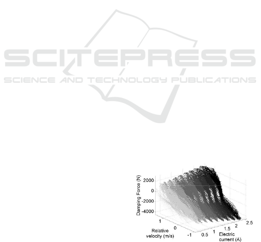
several needs. Figure 1 shows the highly nonlinear

behavior of an industrial MR damper under various

constant electric current inputs, its accurate modeling

is a non-trivial task.

Figure 1: Nonlinear behavior of the MR damper force re-

spect to the control current and relative velocity.

Several mathematical models are available for

modeling the nonlinear behavior of MR dampers;

generally, they can be grouped as parametric and

non-parametric models. Parametric models in-

clude the Bingham model (Stanway et al., 1987),

493

C. Tudón-Martínez J., Morales-Menendez R., A. Ramirez-Mendoza R. and E. Garza-Castañón L..

MR Damper Identiﬁcation using ANN based on 1-Sensor - A Tool for Semiactive Suspension Control Compliance.

DOI: 10.5220/0004159004930502

In Proceedings of the 4th International Joint Conference on Computational Intelligence (NCTA-2012), pages 493-502

ISBN: 978-989-8565-33-4

 2012 SCITEPRESS (Science and Technology Publications, Lda.)

the viscoelastic-plastic model (Gamota and Filisko,

1991), the phenomenological model (Wang and

Kamath, 2006), the semi-phenomenological model

based on the BoucWen model (Spencer et al., 1996),

the improved BoucWen model (Yang et al., 2002),

the hyperbolic tangent function model (Kwok et al.,

2006), (Guo et al., 2006), the inverse tangent func-

tion model (C¸ esmeci and Engin, 2010) and many oth-

ers. The Bingham and the viscoelastic-plastic model

can not reproduce the nonlinear behavior of an MR

damper with high accuracy, while the other models

can; however, they have many parameters to identify.

On the other hand, some of these physical models use

parameters of the internal structure of the shock ab-

sorber resulting a particular model case.

In the non-parametric models, the coefﬁcients do

not have a physical meaning. Models based on look-

up table, fuzzy logic and Artiﬁcial Neural Networks

(ANN) are the representative non-parametric models

for a MR damper. Polynomial models [(Choi et al.,

2001), (Hong et al., 2002), (Du et al., 2005), (Poussot-

Vassal et al., 2008)] require many parameters to ex-

press the nonlinear and semiactive behavior of the

damping force; while the fuzzy models [(Atray and

Roschke, 2003), (Ahn et al., 2008)] need a priori

knowledge in the frequency and time domain of the

MR damper. For ANN models, the knowledge of the

dynamic relationships between the variables is not re-

quired, only a well training step is needed; in addi-

tion, the number of parameters depends on the struc-

ture size and commonly the ANN design is based on

the minimal dimensions criterion (Freeman and Ska-

pura, 1991), which selects the possible lowest number

of hidden layers with the possible lowest number of

neurons.

The major effort in the MR damper modeling, by

using ANN, is focused on reproduce the inverse dy-

namics (force-electric current) of the shock absorber

(Chang and Zhou, 2002), (Zapateiro et al., 2009),

(Metered et al., 2010); however, a recurrent neural

network is required for achieving an optimal damping

force signal, and normally the input vector is based on

two or more sensor measurements: force, displace-

ment and/or velocity. This type of ANN model in-

creases the architecture size and the instrumentation

cost in a suspension control system. On the other

hand, commonly the modeling of the forward dynam-

ics using ANN requires two ore more time delays of

each input by increasing the ANN architecture and its

computing time (Savaresi et al., 2005), (Chen et al.,

2009), (Boada et al., 2011).

This paper proposes a non-parametricmodel of an

MR damper based on ANN, the model does not require

regressors in the input vector and demands only one

sensor, i.e. its structure has low complexity for prac-

tical implementations of suspension control systems.

The MR damper model is validated with experimen-

tal data of two MR dampers for analyzing its reliabil-

ity and it is used in a suspension control system of a

Quarter of Vehicle (QoV), this is an example of an ap-

plication problem where the accurate modeling of the

actuation device is one of the most crucial part of the

whole control design problem.

The outline of this paper is as follows: in the next

section, the ANN design is described. Section 3 shows

the experimental system and section 4 presents the

modeling results. Section 5 presents the effectiveness

of an MR damper versus a passive damper in compli-

ance of a suspension control system. Conclusions are

presented in section 6.

Table 1: Deﬁnition of variables.

Variable Description

MR damper force

de f

Damper piston position

˙z

de f

Damper piston velocity

I Electric current

Time delays

Sprung mass in the QoV

Unsprung mass in the QoV

Road proﬁle

Vertical position of m

˙z

Vertical velocity of m

˙z

Vertical velocity of m

¨z

Vertical acceleration of m

¨z

Vertical acceleration of m

Spring stiffness coefﬁcient

Wheel stiffness coefﬁcient

2 ANN REVIEW

An ANN is a computational model capable to learn

behavior patterns of a process, it can be used to model

nonlinear, complex and unknown dynamic systems,

(Korbicz et al., 2004). Based on the ﬂow of signals,

the ANN architecture can be classiﬁed into two major

groups: feedforward and recurrent networks. Feed-

forward networks project the ﬂow of information only

in one way, i.e. the output of a neuron feeds to all

neurons of the following layer (Hagan et al., 1996);

while, the recurrent networks have an output feedback

signal.

In MR damper modeling using ANN, typically

recurrent neural networks based on Nonlinear-ARX

(NARX) structures, i.e. regressors in the input and/or

output vector, have been proposed with high accuracy

(Chang and Zhou, 2002), (Savaresiet al., 2005), (Zap-

IJCCI2012-InternationalJointConferenceonComputationalIntelligence

494

ateiro et al., 2009), (Chen et al., 2009), (Metered et al.,

2010), (Boada et al., 2011). The NARX structure is

deﬁned as,

= f

de f

(t), z

de f

(t − 1), . . . , z

de f

(t −k

˙z

de f

(t), ˙z

de f

(t −1), . . . , ˙z

de f

(t −k

I(t), I(t − 1), . . . , I(t − k

(t − 1), . . . , F

(t −k

))

(1)

where k

represents a speciﬁc number of time de-

lays for each signal, z

def

and ˙z

def

are the displacement

and velocity of the damper rod provided from sensor

measurements, I is the actuation signal and F

is the

damper force (ANN output).

In this paper, a comparison between a feedforward

and recurrent neural network is considered for deter-

mining the accuracy degree in the damper force by

adding the output feedback in the ANN structure. In

addition, different arrays in the input vector are used

to evaluate the ANN performance with time delays;

the arrays with one, two and three regressors in the

input vector are compared with the modeling perfor-

mance of an ANN that does not have delays. Finally,

the ANN performance is analyzed when one (velocity)

or two (displacement and velocity) signals are used in

the input vector.

The ANN training is deﬁned as the adaptation pro-

cess of the synaptic connections under external stim-

ulations. The backpropagation algorithm is the most

used training method since it allows to solve prob-

lems with complex net connections; its formulation

can be reviewed in detail in (Freeman and Skapura,

1991). The proposed ANN model was trained with

backpropagation and crossed validation was used to

validate the results.

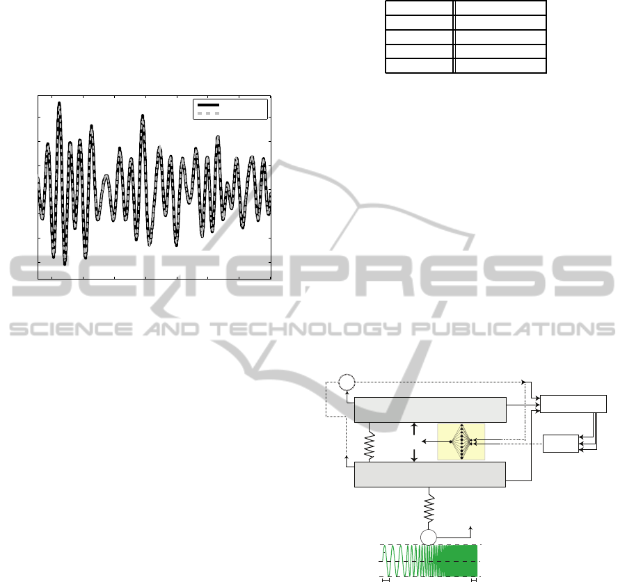
3 EXPERIMENTAL SYSTEM

Two different MR dampers have been used to perform

a total of 5 tests. One damper, called MR

damper,

is designed by Delphi MagneRide

; it has continu-

ous actuation and considerable hysteresis at high fre-

quencies with high deﬂections. The other MR damper,

named MR

damper, is manufactured by BWI

; it

has only two levels of actuation and its hysteretic be-

havior is minimal.

An MTS-407

controller has been used to con-

trol the position of the damper piston, Figure 2. An

NI-9172

data acquisition system commands the

controller and records the position, velocity and force

from the MR damper. A sampling frequency of 1650

Hz was used. The bandwidth of displacement was

0.5- 15 Hz, which lies within comfort and road hold-

ing automotive applications. The displacement and

electric current ranges were: ±25 mm and 0 - 2.5 A,

respectively.

Figure 2 also shows the used sensor (VP510-10

of UniMeasure

), which provides the velocity (˙z

def

)

and position (z

def

) measurements of the damper pis-

ton. In this case, a self-generating tachometer gener-

ates the velocity measurement; however, it is possible

to use another linear velocity transducer.

MTS System

Position and

velocity sensor

MR damper

Figure 2: Experimental system.

A series of training sequences have been proposed

in (Lozoya-Santos et al., 2009), the position emulates

the suspension deﬂection and the electric current is

the actuation signal. Table 2 shows the design of ex-

periments used to identify the nonlinear behavior of

both MR dampers under different sequences of posi-

tion and actuation.

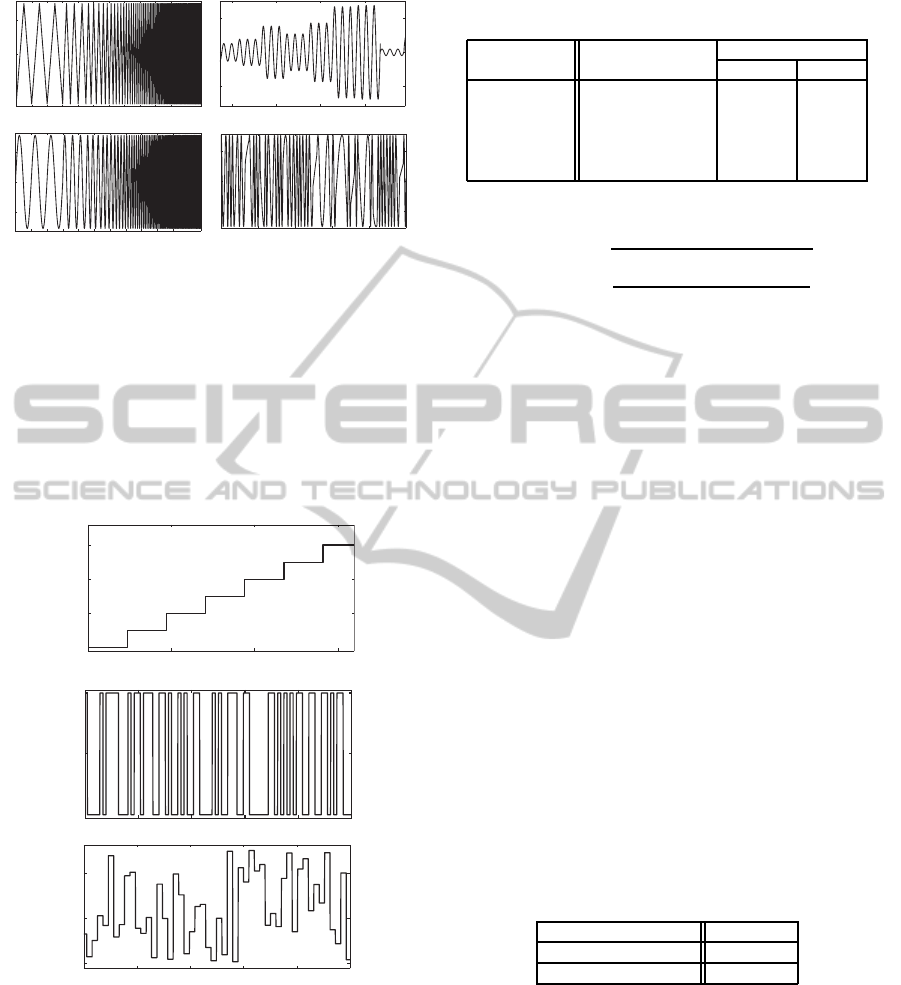
For displacement sequences, Amplitude-

Modulated (AM), Frequency-Modulated (FM)

and Stepped Frequency Sinusoidal (SFS) were used

to analyze the MR damper dynamics in the transient

response under changes in magnitude and frequency

of the suspension deﬂection; Triangular wave with

Positive and Negative Variable Slopes (TPNVS)

sequence allows to know the dynamic behavior under

constant velocity; and Road Proﬁle (RP) represents

the suspension deﬂection move when the vehicle

passes under a speciﬁc surface. Figure 3 presents

some of the different displacement sequences used

in the experimental stage in order to identify the

nonlinear behavior of both MR dampers.

For electric current sequences, Stepped inCre-

ments (SC) are used to study the effect of the current

in the jounce and rebound of the MR damper under

different displacements, since the MR

damper has

not a continuous actuation only two levels of current

were designed; Increased Clock Period Signal (ICPS)

and Pseudo Random Binary Signal (PRBS) allow to

analyze the transient response of the damping force

MRDamperIdentificationusingANNbasedon1-Sensor-AToolforSemiactiveSuspensionControlCompliance

495

2 4 6 8 10 12 14 16 18 20

-20

Displacement (mm)

2 10 20

-20

Displacement (mm)

36 40 44 48

-20

TPNVS

SFS

11 12 13 14 15

-20

Time (s)

Figure 3: Displacement sequences in the piston used in the

experimental stage.

when the current changes at different frequencies, the

ICPS signal includes random changes in the ampli-

tude and PRBS only switches between two electric

current values. Figure 4 shows the behavior of the

actuation sequences used in the experiments, for the

damper, the SC sequence only has two states: 0

and 2.5 A.

0 50 100 150

0.6

1.2

2.5

Electric Current (A)

11 12 13 14

Electric Current (A)

ICPS

6 7 8 9

2.5

PRBS

Time (s)

Electric Current (A)

Figure 4: Electric current sequences used in the experimen-

tal stage.

4 MODELING RESULTS

The ANN model obtained from the different experi-

ments, presented in Table 2, is used to characterize

the dynamical behavior of the MR damper and eval-

uated by the Root Mean Square (RMS) performance

Table 2: Design of experiments for identifying an MR

damper.

Experiment Displacement Current sequence

sequence MR

1 TPNVS SC (10) SC (2)

2 SFS SC (10) SC (2)

3 RP (rough way) ICPS PRBS

4 AM ICPS PRBS

5 FM ICPS PRBS

index of the error, which is deﬁned as,

RMS =

∑

i=1



(i) − F

(i)



(2)

where,

and F

represent the estimated and ex-

perimental damping force respectively and n is the

number of total samples in the experiment. The per-

centage of error represents the RMS of the error nor-

malized by the span of the damping force.

First, the design issues for the ANN model are dis-

cussed: the network structure, the required sensors in

the input vector, the regressor choice and the selection

of the number of parameters of the ANN.

Remark: ANN architecture. A Multilayer Percep-

tron (MLP) network, which corresponds to a feedfor-

ward system, is compared with a recurrent network.

The input vector of the MLP network is composed

by z

def

, ˙z

def

, I; while the recurrent network adds the

ANN output (damping force). Table 3 presents the

modeling error of both structures by using the exper-

iment 2 in the MR

damper as example. The error

percentage represents the average deviation between

the modeled damping force and the real measurement

based on the RMS value of the error. When the feed-

back of the MR damper force is considered, the mod-

eling error decreases slightly; however, the ANN ar-

chitecture and its computing time increase.

Table 3: Performance comparison between the feedforward

and recurrent neural networks.

ANN Structure Error (%)

MLP (feedforward) 4.38

Recurrent 3.80

Remark: Sensors in the Input Vector. Taking into

account an MLP network, two different input vectors

have been compared. The former input vector uses

the z

def

, ˙z

def

and I; while the second one only in-

cludes ˙z

def

and I. Table 4 indicates that the model-

ing error decreases 46.7 % by considering two sensor

measurements in addition to the electric current sig-

nal; however, the instrumentation cost can increase

and the ANN structure is more complex for the train-

ing and testing step.

IJCCI2012-InternationalJointConferenceonComputationalIntelligence

496

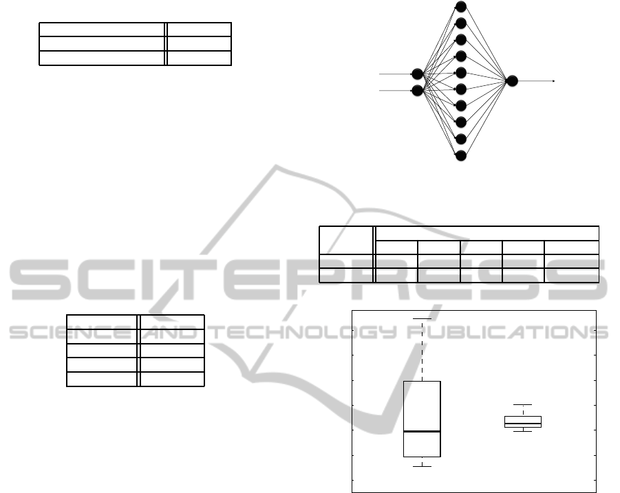
Table 4: Modeling error (%) in the MLP network using dif-

ferent input vectors.

Sensor Measurements Error (%)

1 (˙z

de f

) 8.22

2 (z

de f

and ˙z

de f

) 4.38

Remark: Regressor Choice. Once the ANN archi-

tecture and the input vector are deﬁned, different ar-

rays in the input vector of the ANN model have been

evaluated, in this case the experiment 2 over the MR

damper is used as example. Table 5 shows the model-

ing error of the ANN when the number of regressors

in the 2 input signals varies; in this analysis, the ve-

locity and electric current have the same number of

regressors in each test. According to the modeling er-

ror, it is not signiﬁcant to incorporate time delays in

the input vector of the ANN.

Table 5: Modeling error (%) in the ANN with different num-

ber of regressors in the input vector.

Regressors Error (%)

0 8.22

1 8.24

2 8.86

3 8.79

Remark: ANN-size Selection. Finally, the choice of

the number of parameters (hidden layers and neurons

in these layers) of the non-linear parametric function

can be easily made using a cross-validation approach.

A 1-hidden-layer structure has been chosen by sim-

ulation tests, this structure guarantees the universal-

approximation property (Sj¨oberg, 1995). For deter-

mining the number of neurons in the hidden layer, the

minimal dimensions criterion is used (Freeman and

Skapura, 1991); the best choice is with 10 neurons.

According to the above design issues, the ANN ar-

chitecture used to model the MR damper dynamics is

(2,10,1), Figure 5. The ANN input vector includes the

signal of the relative velocity and the excitation sig-

nal (electric current) without considering regressors,

while the damping force corresponds to the ANN out-

put. Modeling results of the proposed ANN model,

considering the 5 experiments, is shown in the Table

6. Figure 6 shows the variability of the modeling re-

sults. Clearly, the variance of the error is greater in the

model of the MR

damper since its continuous actu-

ation adds more nonlinearities, which complicate the

modeling task; while, the MR

damper model shows

better modeling performance with lower error stan-

dard deviation of the error.

The RMS average, considering all experiments, is

291.4 N for the MR

damper and 597.8 N for the

damper. Since the span of the force is ±4000

Displacement or

velocity sensor

Electric

Curre

Input

layer

Output

layer

Hidden layer

Figure 5: Feedforward ANN of the MR damper model.

Table 6: Modeling error in different experimental tests.

MR Experiment

damper 1 2 3 4 5

5.9% 8.2% 3.1% 4.1% 14.95%

6.9% 6.8% 7.2% 8.0% 6.2%

Percentage of error

1 2

Figure 6: Variability of the error in the MR damper models.

N approximately for the MR

damper and [−6000 to

11000] N for the MR

damper, the obtained RMS av-

erage represents the 7.25% and 7.02% of punctual er-

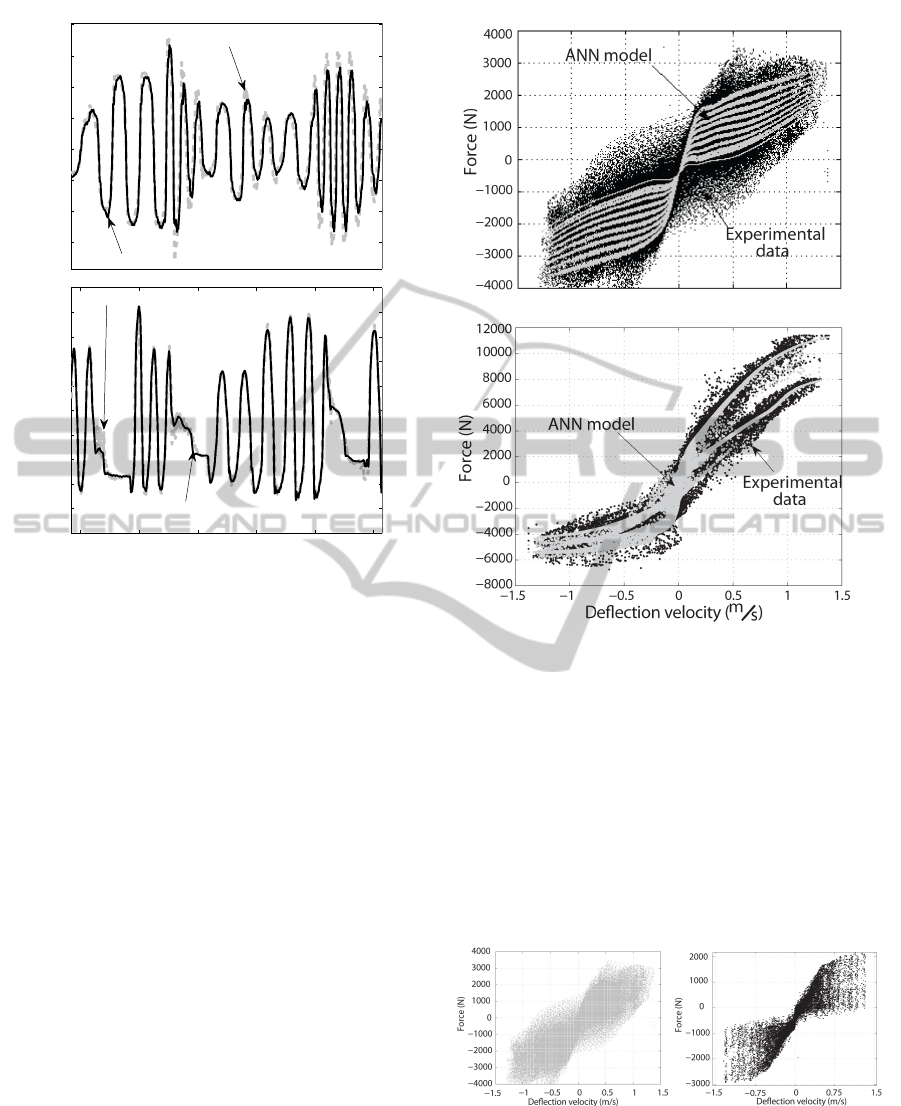
ror in the force signal, respectively. Figure 7 presents

a qualitative comparison in the transient response of

the force obtained from experimental data and from

ANN model; in this case, the MR

and MR

dampers

are subject to the experiment 5. According to Table

6, the MR

damper has greater modeling error in the

experiment 2 and 5, and viceversa.

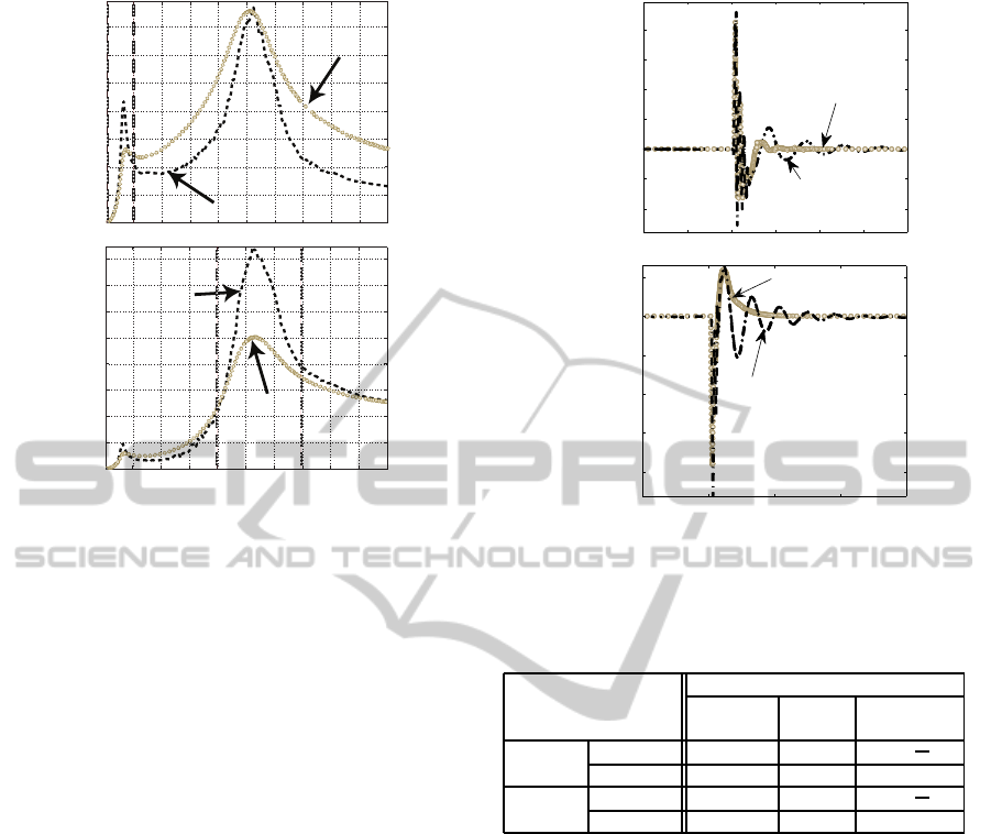
In order to test the capability of the ANN for

modeling the nonlinear and hysteretic behavior of the

MR damper, experimental data are compared with the

ANN model in the characteristic diagram of Force-

Velocity (FV); this diagram explains the effect of

jounce and rebound of the damper and it is a tool for

the engineers of automotive design in order to deﬁne

the suspension capability for improving the confort

and road holding. Figure 8 shows the FV diagram of

MRDamperIdentificationusingANNbasedon1-Sensor-AToolforSemiactiveSuspensionControlCompliance

497

0.95 1 1.05 1.1 1.15 1.2

x 10

−8000

−6000

−4000

−2000

2000

4000

6000

8000

10000

12000

Samples

Force (N)

ANN model

Experimental data

−3000

−2000

−1000

1000

2000

3000

4000

Force ( N)

Experimental data

ANN model

Figure 7: Comparison between the real and modeled force

using the MR

damper (up) and MR

damper (bottom).

both dampers using the experiment 2. Bottom plot

in Figure 8 shows that the ANN can model the non-

linear behavior of the MR

damper with acceptable

accuracy, only outliers are not included. Notice in the

FV diagram that the MR

damper has minimal hys-

teresis and it is composed by two damping leves: 1)

high damping force at current greater than 2.5 A and

2) low damping force at 0 A. On the other hand, the

damper has a continuous actuation between 0

and 2.5 A. The ANN correctly models the nonlinear

behavior at each current step; however, the hystere-

sis can not be modeled at low deﬂection velocities

(±0.5 m/s) using only one sensor, up plot in Figure

8. This hysteretic behavior occurs at high frequencies

(greater than 10 Hz) with high amplitudes in the sus-

pension deﬂection, and the velocity sensor does not

contain the required information for representing the

force dynamics at these frequencies; thus, an accel-

eration sensor could complement this missing force

dynamics.

Although the hysteresis can not be modeled at

high frequencies with high displacements, in general,

the proposed ANN can be used to represent the MR

damper dynamics since the hysteretic behavior ap-

pears at not typical deﬂection amplitudes in an auto-

motive suspension and the frequencies out of the de-

sired span for passengers comfort, i.e. the position

Figure 8: FV diagram for the real and modeled force using

the MR

damper (up) and MR

damper (bottom).

pattern is out of the automotive operational zone of

the damper. Figure 9 shows the comparison of the

FV diagram using experimental data provided from

the experiment 2 (left plot) and 4 (right plot). Since

the experiment 4 contains data at high frequencies but

low amplitudes on the displacement, the hysteresis

phenomenon is minimal; while, the experiment 2 has

high displacements at high frequencies that cause too

much hysteresis.

Figure 9: FV diagram for the MR

damper using experi-

mental data from experiment 2 (left) and 4 (right).

Another form of getting the ANN model of the MR

damper is by using the estimated deﬂection velocity

through a displacement sensor. Figure 10 shows that

the measurement of the deﬂection velocity is prac-

IJCCI2012-InternationalJointConferenceonComputationalIntelligence

498

tically similar to the estimated signal, in this case

the central differentiation algorithm over the displace-

ment measurement is considered. Therefore, it can

be used a displacement or velocity sensor, additional

to the actuation signal, for achieving a reliable MR

damper model based on ANN.

1.2 1.3 1.4 1.5 1.6 1.7 1.8 1.9

x 10

−0.6

−0.4

−0.2

0.2

0.4

0.6

Samples

Deection velocity [m/s]

Measurement

Estimation

Figure 10: Comparison between the real and estimated de-

ﬂection velocity for the experiment 3 in the MR

damper.

5 MR DAMPER USED IN

AUTOMOTIVE SUSPENSIONS

In order to analyze the effectiveness of the MR

damper model based on ANN, a semiactive suspen-

sion control system of a QoV model is used as test-

bed; the ANN model is included for increasing the

comfort of passengers maintaining the road holding.

The QoV model considers a sprung mass (m

) and

an unsprung mass (m

). A spring with stiffness co-

efﬁcient k

and a MR damper represent the suspen-

sion between both masses. The stiffness coefﬁcient k

models the wheel tire. The vertical position of the

mass m

) is deﬁned by z

), while z

cor-

responds to the road proﬁle. It is assumed that the

wheel-road contact is ensured.

The system dynamics is given by,

¨z

= −k

− z

) − F

(3)

¨z

= k

− z

) − k

− z

) + F

(4)

where, F

is the MR damping force obtained by the

ANN model, which is based on the MR

damper dy-

namics. The QoV model parameters described in 3

and 4 have been identiﬁed on a commercial vehicle,

Table 7.

The MR force depends on the deﬂection velocity

˙z

def

= ˙z

− ˙z

and electric current I, this later signal

represents the controller output. Several approaches

Table 7: QoV model parameters of a commercial vehicle.

Parameter Value

387 (Kg)

139.5 (Kg)

37,300 (N/m)

295,200 (N/m)

in control of semiactive suspensions have been pro-

posed (Dong et al., 2010), (Spelta et al., 2010), etc.

The comfort performance of a semiactive sus-

pension, using the Mix 1-sensor (Mix1) control law,

is compared with a commercial vehicle suspension

which uses a passive damper. Experimental data

of the passive damper were modeled by the same

ANN technique as the semiactive dampers. Figure 11

shows a conceptual diagram of the semiactive suspen-

sion control system; the ANN model, which has been

trained off-line, only requires the deﬂection velocity

and the electric current for generating the MR force in

a forward way. The block of processing of signals in-

cludes ﬁlters, estimators and/or observers in order to

achieve the control law. Details on the Mix1 control

law can be reviewed in (Spelta et al., 2010).

def

peak

(mm)

. .

peak

Processing of signals

Controller

0.5 Hz

20 Hz

Figure 11: General structure of semiactive suspension con-

trol system.

In order to analyze the passengers comfort and

road holding in the frequency and time domain, two

road disturbance inputs have been simulated: 1) in the

frequency domain, a signal chirp of 2 cm with span

of [0.5-20]Hz and 2) in the time domain, a step of 3

cm. Figure 12 shows the QoV performance in the fre-

quency domain; the Power Spectral Density (PSD) is

used as performance index, i.e. the maximum gain of

a signal is plotted at any speciﬁc frequency. The fre-

quency response of the QoV model with the passive

damper is considered as benchmark.

According to (Poussot-Vassal et al., 2008), Fig-

ure 12 shows that the controller fulﬁlls with the per-

MRDamperIdentificationusingANNbasedon1-Sensor-AToolforSemiactiveSuspensionControlCompliance

499

2 4 6 8 10 12 14 16 18 20

100

150

200

250

300

350

gain

2 4 6 8 10 12 14 16 18 20

0.5

1.5

2.5

3.5

frequency [Hz]

gain

Mix-1

passive

Comfort z

Road Holding z - z

us r

Mix-1

passive

Figure 12: Frequency response of the QoV model in closed-

loop using a semiactive and passive suspension, the span of

frequencies of interest for each objective is bounded by the

vertical discontinuous lines.

formance speciﬁcation for comfort: at low frequen-

cies [0-2]Hz, the maximum gain of ¨z

respect to the

surface is lower than the passive suspension. In this

range of frequencies, a human can feel dizziness and

sickness caused by sudden motions. On the other

hand, a good road holding is considered when the

maximum gain of z

− zr respect to z

is limited to

2.5 for low disturbances (z

< 3cm) between 0 to 20

Hz, specially close to the resonance frequency of m

Bottom plot in Figure 12 indicates that the semiac-

tive suspension control system has good road hold-

ing performance in all span of frequencies, the PSD

reduces until 2 units in the resonance frequency of

the unsprung mass. Thus, the road holding increases

40.4% by using a semiactive suspension system.

For the time domain, the effectiveness of the semi-

active suspension versus the passive suspension is

clear. Figure 13 displays the transient response of

the acceleration of the sprung mass (up plot) and of

the wheel deﬂection (bottom plot). In both transient

responses, the semiactive control system can reduce

more of 50% in the settling time and decay ratio and

approximately a 10% of the the maximum deviation,

Table 8. Taking into account the RMS of the ¨z

signal,

the comfort increases 7.4% with the Mix1 controller.

For road holding, the Mix1 controller improves 64.9%

respect to he passive suspension.

500 1000 1500 2000 2500 3000

−2

−1

1000 2000 3000 4000

−0.04

−0.03

−0.02

−0.01

0.01

Samples

Passive

Mix 1

Passive

Comfort z

Road Holding z - z

us r

(m)

(m/s )

Figure 13: Transient response of the QoV model in closed-

loop using different automotive suspension schemes.

Table 8: Performance in the transient response of the sus-

pension control system.

Suspension Performance Index

Control Settling Decay Maximum

System Time (s) Ratio Deviation

Semi- Comfort 0.3 0.07 4.1

active Holding 0.6 0 -3.8cm

Passive Comfort 0.8 0.15 4.5

Holding 1.7 0.23 -4.5cm

6 CONCLUSIONS

A Magneto-Rheological (MR) damper model based

on Artiﬁcial Neural Networks (ANN) is proposed.

The ANN structure does not require regressors in the

input vector and only one sensor (displacement or ve-

locity) is demanded to get a reliable model. In addi-

tion, it has been proved that the output feedback in the

input vector of the ANN model only improves slightly

the modeling performance; however, the computing

time in the training and testing step increases because

the ANN architecture requires more model parameters

when the output feedback is included.

Experimental data provided from two MR

dampers (Delphi

named MR

damper, and BWI

named MR

damper) with different properties have

been used to verify the accuracy of the proposed MR

damper model based on ANN. The average modeling

error in the force signal is lower than 7.25% by con-

IJCCI2012-InternationalJointConferenceonComputationalIntelligence

500

sidering 5 different experiments. The force-velocity

diagram shows that the MR

damper can be mod-

eled with high accuracy by the proposed ANN struc-

ture since this shock absorber has an on/off actuation

and does not have hysteresis; while the MR

damper

presents a more complex dynamics at high frequen-

cies with high displacements and the MR damper

model based on the proposed 1-hidden layer structure

can not represent this hysteretic behavior with only

one sensor. However, this displacement pattern is out

of the automotive operational zone of the damper, i.e.

it does not occur at normal driving conditions.

By comparing the modeling performance of the

proposed MR damper model based on ANN with an-

other MR damper models presented in the literature,

it is considerable to assume an optimal modeling per-

formance. In the proposed ANN model, the obtained

modeling error of 7.25% based on the RMS is equiv-

alent to 4.7% of Error to Signal-Ratio (ESR), this

means that the error in the proposed ANN model

is: 1) lower than the ESR average (14.5%) obtained

by the Bingham model and reported in (Savaresi

et al., 2005); 2) lower than the ESR average (8.7%)

obtained by a phenomenological model reported in

(Ruiz-Cabrera et al., 2010); lower than the ESR av-

erage (38.7%) obtained by a semi-phenomenological

model reported in (Ruiz-Cabrera et al., 2010); but

greater than the ESR average of (0.9%) and (2%) ob-

tained by an ANN model reported in (Savaresi et al.,

2005) and (Ruiz-Cabrera et al., 2010) respectively.

Although these latter ANN structures have regressors,

use the output feedback and demand the displacement

and velocity sensor.

Due to reliability of the proposed MR damper

model and simplicity on the ANN structure, the model

can be used to test semiactive suspension control sys-

tems. A control technique free of model has been

used to control the semiactive suspension of a quar-

ter of vehicle system; the performance of the passive

suspension was used as benchmark. Simulation re-

sults show that passengers comfort and road holding

can be increased at least 7.4% and 40.4% respectively,

when an MR semiactive suspension is used.

ACKNOWLEDGEMENTS

Authors thank to CONACYT (Program of Postgradu-

ate Cooperation - 2010) for the ﬁnancial supports of

this research.

REFERENCES

Ahn, K., Islam, M., and Truong, D. (2008). Hysteresis

modeling of magneto-rheological (mr) ﬂuid damper

by self tuning fuzzy control. In ICCAS 2008, Seoul

Korea, pages 2628–2633.

Atray, V. and Roschke, P. (2003). Design, fabrica-

tion, testing and fuzzy modeling of a large magneto-

rheological damper for vibration control in a railcar.

In IEEE/ASME Joint Rail Conf., pages 223–229.

Boada, M., Calvo, J., Boada, B., and D´ıaz, V. (2011). Mod-

eling of a magnetorheological damper by recursive

lazy learning. International Journal of Non-Linear

Mechanics, 46:479–485.

C¸ esmeci, S. and Engin, T. (2010). Modeling and test-

ing of a ﬁeld-controllable magnetorheological ﬂuid

damper. International Journal of Mechanical Sci-

ences, 52(8):1036–1046.

Chang, C. and Zhou, L. (2002). Neural network emulation

of inverse dynamics for a magnetorheological damper.

Journal of Structural Engineering, 128(2):231–239.

Chen, E., Si, C., Yan, M., and Ma, B. (2009). Dy-

namic characteristics identiﬁcation of magnetic rhe-

ological damper based on neural network. In Ar-

tiﬁcial Intelligence and Computational Intelligence,

2009, Shangai, China, pages 525–529.

Choi, S., Lee, S., and Park, Y. (2001). A hysteresis

model for ﬁeld-dependent damping force of a mag-

netorheological damper. J. of Sound and Vibration,

245(2):375–383.

Dong, X., Yu, M., Liao, C., and Chen, W. (2010). Com-

parative research on semi-active control strategies for

magneto-rheological suspension. Nonlinear Dynam-

ics, 59:433–453.

Du, H., Szeb, K., and Lam, J. (2005). Semiactive h

con-

trol of vehicle suspension with magneto-rheological

dampers. J. of Sound and Vibration, 283:981–996.

Freeman, J. and Skapura, D. (1991). Neural Networks: Al-

gorithms, Applications and Programming Techniques.

Adisson-Wesley.

Gamota, D. and Filisko, F. (1991). Dynamic mechanical

studies of electrorheological materials: Moderate fre-

quencies. Journal of Rheology, 35:399–425.

Guo, S., Yang, S., and Pan, C. (2006). Dynamical modeling

of magneto-rheological damper behaviors. Int. Mater.,

Sys. and Struct., 16:3–14.

Hagan, M., Demuth, H., and Beale, M. (1996). Neural Net-

work Design. PWS Publishing.

Hong, K., Sohn, H., and Hedrick, J. (2002). Modi-

ﬁed skyhook control of semi-active suspensions: A

new model, gain scheduling, and hardware-in-the-

loop tuning. J. Dyn. Sys., Meas., Control, 124(1):158–

167.

Korbicz, J., Koscielny, J., Kowalczuk, Z., and Cholewa,

W. (2004). Fault Diagnosis Models, Artiﬁcial Intel-

ligence, Applications. Springer.

Kwok, N., Ha, Q., Nguyen, T., Li, J., and Samali, B. (2006).

A novel hysteretic model for magnetorheological ﬂuid

dampers and parameter identiﬁcation using particle

MRDamperIdentificationusingANNbasedon1-Sensor-AToolforSemiactiveSuspensionControlCompliance

501

swarm optimization. Sensors and Actuators A: Physi-

cal, 132:441–451.

Lozoya-Santos, J., Morales-Menendez, R., and Ramirez-

Mendoza, R. (2009). Design of experiments for mr

damper modelling. In 17th Int. Joint Conf. on Neural

Networks, pages 1915–1922.

Metered, H., Bonello, P., and Oyadiji, S. (2010). The exper-

imental identiﬁcation of magnetorheological dampers

and evaluation of their controllers. Mechanical Sys-

tems and Signal Processing, 24:976–994.

Poussot-Vassal, C., Sename, O., Dugard, L., G´asp´ar, P.,

Szab´o, Z., and Bokor, J. (2008). A new semi-active

suspension control strategy through lpv technique.

Control Engineering Practice, 16(12):1519–1534.

Ruiz-Cabrera, J., D´ıaz-Salas, V., Morales-Menendez, R.,

n´on, L. G.-C., and Ramirez-Mendoza, R. (2010).

Comparison of mr damper models. In 18th Mediter-

ranean Conference on Control and Automation, Mar-

rakech Morocco, June 23-25, pages 1509–1513.

Savaresi, S., Bittanti, S., and Montiglio, M. (2005). Iden-

tiﬁcation of semi-physical and black-box non-linear

models: the case of mr-dampers for vehicles control.

Automatica, 41:113–127.

Sj¨oberg, J. (1995). Non-linear System Identiﬁcation with

Neural Networks. PhD thesis, Link¨oping University,

Sweden.

Spelta, M., Savaresi, S., and Fabbri, L. (2010). Experi-

mental analysis of a motorcycle semi-active rear sus-

pension. Control Engineering Practice, article in

press:doi:10.1016/j.conengprac.2010.02.006.

Spencer, B., Dyke, S., Sain, M., and Carlson, J. (1996). Phe-

nomenological model of a mr damper. ASCE Journal

of Engineering Mechanics, 123(3):230–238.

Stanway, R., Sproston, J., and Stevens, N. (1987). Non-

linear modeling of an electrorheological vibration

damper. Journal of Electrostatics, 20:167–184.

Wang, L. and Kamath, H. (2006). Modeling hysteretic

behaviour in mr ﬂuids and dampers using phase-

transition theory. Smart Mater. Struct., 15:1725–1733.

Yang, G., Jr., B. S., and Dyke, S. (2002). Large-scale mr

ﬂuid dampers: Modeling and dynamic performance

considerations. Engineering Structures, 24:309–323.

Zapateiro, M., Luo, N., Karimi, H., and Veh´ı, J. (2009).

Vibration control of a class of semiactive suspension

system using neural network and backstepping tech-

niques. Mechanical Systems and Signal Processing,

23:1946–1953.

IJCCI2012-InternationalJointConferenceonComputationalIntelligence

502