Transonic Wing Optimization by Variable-resolution Modeling

and Space Mapping

Eirikur Jonsson, Leifur Leifsson and Slawomir Koziel

Engineering Optimization & Modeling Center, School of Science and Engineering, Reykjavik University, Reykjavik, Iceland

Keywords:

Transonic Wing Design, CFD, Surrogate-based Optimization, Variable-resolution Modeling, Space Mapping.

Abstract:

This paper presents an efﬁcient aerodynamic design optimization methodology for wings in transonic ﬂow.

The approach replaces the computationally expensive high-ﬁdelity CFD model in an iterative optimization

process with a corrected polynomial approximation model constructed by a cheap low-ﬁdelity CFD model.

The output space mapping technique is used to correct the approximation model to yield an accurate predictor

of the high-ﬁdelity one. Both CFD models employ the RANS equations with the Spalart-Allmaras turbulence

model, but the low-ﬁdelity one uses a coarse mesh resolution and relaxed convergence criteria. Our method

is applied to a constrained lift maximization of a rectangular wing at transonic conditions with 3 design vari-

ables. The optimized designs are obtained by using 50 low-ﬁdelity CFD model evaluations to set up the

approximation model and 7 to 8 high-ﬁdelity model evaluations, equivalent to around 10 high-ﬁdelity CFD

model evaluations.

1 INTRODUCTION

The wing is the most important component of an air-

craft, signiﬁcantly affecting its overall performance.

As the wing provides lift, it is at the same time the

main source of drag, responsible for about 2/3 of the

total drag of the aircraft (Raymer, 2006). Reducing

this wing drag by a better design, and, hence, mini-

mizing cost, is often the primary objective of modern

aircraft design.

Nowadays, aerodynamic design using high-

ﬁdelity computational ﬂuid dynamic (CFD) models

is ubiquitous and plays an important role in aircraft

development. Traditional design optimization tech-

niques, such as gradient-based or population-based

ones, involve a large number of simulations. Conse-

quently, direct aerodynamic optimization with high-

ﬁdelity CFD models using traditional optimization

techniques is impractical, even when using cheap ad-

joint sensitivities.

One of the overall objectives of surrogate-based

optimization (SBO) (Queipo et al., 2005; Forrester

and Keane, 2009) is to reduce the number of evalu-

ations of expensive simulations, thereby making the

design process more efﬁcient. This is achieved by an

iterative correction-prediction process where a surro-

gate model (a computationally cheap representation

of the high-ﬁdelity one) is constructed and subsequen-

tly exploited to obtain approximate location of the

high-ﬁdelity model optimal design. The surrogate

model can be constructed by approximating sampled

high-ﬁdelity model data using, e.g., polynomial ap-

proximation (Queipo et al., 2005), radial basis func-

tions (Forrester and Keane, 2009; Wild et al., 2008),

kriging (Koziel et al., 2011; Simpson et al., 2001;

Journel and Huijbregts, 1978; O’Hagan and King-

man, 1978), neural networks(Haikin, 1998; Min-

sky and Papert, 1969), or support vector regression

(Smola and Sch

olkopf, 2004) (response surface ap-

proximation surrogates) or by correcting/enhancing

a physics-based low-ﬁdelity model (physical surro-

gates) (Søndergaard, 2003) .

Approximation surrogates usually require a sig-

niﬁcant number of high-ﬁdelity model evaluations to

ensure decent accuracy. Furthermore, the number of

samples typically grows exponentially with the num-

ber of design variables. On the other hand, approx-

imation surrogates can be a basis of efﬁcient global

optimization techniques (Forrester and Keane, 2009).

Various techniques of updating the training data set

(so-called inﬁll criteria (Forrester and Keane, 2009))

have been developed that aim at obtaining global

modeling accuracy, locating globally optimal design,

or the trade-offs between the two, particularly in the

context of kriging interpolation (Forrester and Keane,

2009).

489

Jonsson E., Leifsson L. and Koziel S..

Transonic Wing Optimization by Variable-resolution Modeling and Space Mapping.

DOI: 10.5220/0004164004890498

In Proceedings of the 2nd International Conference on Simulation and Modeling Methodologies, Technologies and Applications (SDDOM-2012), pages

489-498

ISBN: 978-989-8565-20-4

 2012 SCITEPRESS (Science and Technology Publications, Lda.)

Physics-based surrogate models are not as versatile

as approximation ones because they rely on an un-

derlying low-ﬁdelity model (a simpliﬁed description

of the system under consideration), typically prob-

lem speciﬁc. The physics-based models can be ob-

tained by a number of ways, such as by neglecting

certain second-order effects, using simpliﬁed equa-

tions, or, which is probably the most versatile ap-

proach, by exploiting the same CFD solver as used

to evaluate the high-ﬁdelity model but with coarser

mesh and/or relaxed convergence criteria (so called

variable-resolution modeling) (Leifsson and Koziel,

2011b). The physics-based surrogate models contain

knowledge about the system of interest. Due to this,

a limited amount of high-ﬁdelity model data is nec-

essary to ensure a required accuracy of the surrogate.

For the same reason, these physics-based models have

good generalization capabilities.

There have been proposed several SBO algo-

rithms using physics-based surrogates in the litera-

ture, including the approximation and model manage-

ment optimization (AMMO) (Alexandrov and Lewis,

2001), space mapping (SM) (Bandler et al., 2004;

Koziel et al., 2008), manifold mapping (MM) (Echev-

erria and Hemker, 2005), and, more recently, the

shape-preserving response prediction (SPRP) (Leifs-

son and Koziel, 2011a). All of these methods differ in

a speciﬁc way of how the low-ﬁdelity model is used

to construct the surrogate. Space mapping is proba-

bly the most popular approach of this kind. It was

originally developed for simulation-driven design in

microwave engineering (Bandler et al., 2004) how-

ever, it is currently becoming more and more popular

in other areas of engineering and science (cf. Refs.

(Bandler et al., 2004; Koziel et al., 2008), and refer-

ences therein). Despite its potential, space mapping

has not become popular in aerodynamic shape opti-

mization. The only work reported so far is by Robin-

son et al. (Robinson et al., 2006), where the so-called

corrected SM was applied, among other methods, to

airfoil design, however no signiﬁcant design speed up

has been reported.

In this paper, we develop a space mapping al-

gorithm for the aerodynamic design optimization

of wings in transonic ﬂow. In particular, we ex-

tend our recently developed algorithm for airfoils in

two-dimensional transonic ﬂow (Koziel and Leifs-

son, 2012) which employed variable-resolution mod-

els and output space mapping (Bandler et al., 2004;

Koziel et al., 2008). The algorithm proposed in

this work handles three-dimensional ﬂow past wings.

The complicated ﬂuid ﬂow analysis includes a cer-

tain level of numerical noise. To overcome associ-

ated problems, we have replaced the direct use of low-

ﬁdelity models by approximation models. We demon-

strate the effectiveness of the algorithm by a couple of

numerical examples involving constrained lift maxi-

mization.

2 CFD MODELING

In this section, we present the CFD model. In partic-

ular, the governing equations, geometry and grid gen-

eration are presented. We, furthermore, present the

results of a grid convergence study and model valida-

tion.

2.1 Governing Equations

Commercial transport aircraft operate in the transonic

ﬂow regime where the ﬂow is compressible. We as-

sume that the ﬂuid is air modelled by the ideal gas

law and the Sutherland law for dynamic viscosity µ.

The ﬂow is assumed to be steady, viscous, and with-

out body forces, mass-diffusion, chemical reactions

or external heat addition. We solve the RANS equa-

tions with the one equation Spalart-Allmaras turbu-

lence model (Tannehill et al., 1997).

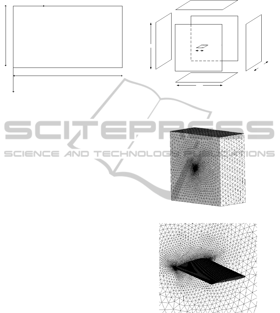
2.2 Wing Geometry

In this work, we consider a simple constant chord

wing. The wing is constructed by two NACA four

digit airfoils (Abbott and Von Doenhoff, 1959), one

at the root and the other at the tip as shown in Fig. 1.

Three parameters deﬁne each airfoil section, namely

the maximum ordinate of the mean camberline as a

fraction of chord (m), the chordwise position of the

maximum ordinate (p), and the thickness-to-chord ra-

tio (t/c) (see Abbott and von Doenhoff (Abbott and

Von Doenhoff, 1959) for details). The reason for

choosing these particular airfoils and the wing geom-

etry is to limit the number of design variables in our

initial study.

2.3 Computational Grid

The farﬁeld is conﬁgured in a box topology where the

wing root airfoil is place in the center of the symme-

try plane with its leading edge placed at the origin

(x,y,z) = (0, 0,0). The farﬁeld extends 100 chord

lengths, 100c, in all directions from the wing, up-

stream, above, below and aft of the wing where the

maximum element size in the ﬂow domain is 11 chord

lengths or 11c. The computational domain is shown

in Fig. 2.

SIMULTECH 2012 - 2nd International Conference on Simulation and Modeling Methodologies, Technologies and

Applications

490

b/2

Wing Root

NACA mpxx airfoil 1

Wing Tip

NACA mpxx airfoil 2

Figure 1: A planform view of a constant chord wing used

in this work. The rectangular wing is constructed by two

NACA airfoils, shown at spanstations 1, the wing root, and

2, the wing tip. Each airfoil has its own set of design pa-

rameters. The wing semispan is b/2.

An unstructured tri/tetra shell grid is created on

all surfaces. The shell grid from the wing is then ex-

truded into the volume where the volume is ﬂooded

with tri/tetra elements. The grid is made dense close

to the wing where it then gradually grows in size as

moving away from the wing surfaces. To capture the

viscous boundary layer an inﬂation layer or a prism

layer is created on the wing surfaces as well. In the

stream-wise direction, the number of elements on the

wing is set to 100 on both upper and lower surface.

The bi-geometric bunching law with a growth ratio of

1.2 is employed in the stream-wise direction over the

wing to obtain a more dense element distribution at

the leading edge and the trailing edge. This is done

in order to capture the high pressure gradient at the

leading edge and the separation at the trailing edge.

The minimum element size of the wing in the stream-

wise direction is set to 0.1%c, and it is located at the

leading and trailing edge. In the span-wise direction

elements are distributed uniformly and number of el-

ements set to 100 over the semi-span. A prism layer

is used to capture the viscous boundary layer. This

layer consists of a number of structured elements that

grow in size normal to the wing surface into the do-

main volume. The inﬂation layer has a initial height

of 5 ×10

−6

c where it is grown 20 layers into the vol-

ume using a exponential growth law with ratio of 1.2.

The initial layer height is chosen so that y

< 1 at

all nodes on the wing. The resulting grid is shown in

Fig. 3.

2.4 Flow Solver

The numerical ﬂuid ﬂow simulations are performed

using the computer code ANSYS FLUENT (ANSYS,

200 c

Symmetry 100 c

Pressure Farfield (PF)

Figure 2: A sketch of the computational domain. All bound-

aries are set as pressure-farﬁeld (PF), a side from the wing

surface, which is a wall type. Symmetry is applied through

the wing center. The wing chord length is denoted by c.

(a)

(b)

Figure 3: A view of of the computational grid, (a) the

farﬁeld grid, and (b) a close-up of the wing shell grid.

2010). The implicit density-based solver is applied

using the Roe-FDS ﬂux type. The spatial discretiza-

tion schemes are set to second order for all vari-

ables, and the gradient information is found using

the Green-Gauss node based method. The residuals,

which are the sum of the L

norm of all governing

Transonic Wing Optimization by Variable-resolution Modeling and Space Mapping

491

equations in each cell, are monitored and checked for

convergence. The convergence criterion for the high-

ﬁdelity model is such that a solution is considered to

be converged if the residuals have dropped by six or-

ders of magnitude, or the total number of iterations

has reached 1000. Also, the lift and drag coefﬁcients

are monitored for convergence.

To reﬂect the compressible nature of this prob-

lem, two types of boundaries are used. The pressure-

farﬁeld is applied to the boundary on all surfaces, ex-

cept where the wing penetrates the symmetry bound-

ary. The boundary types is shown in Fig. 2.

Air is the working ﬂuid at compressible tran-

sonic conditions. The free-stream Reynolds number

is Re

∞,S

= 11.72 × 10

, where S is the reference area,

which in this case is planform area. The Mach number

is set to M

∞

= 0.8395 and the angle of attack is set to

α = 0

◦

. We assume that the ﬂow is calm at its bound-

aries and turbulent viscosity ratio set to µ

/µ

∞

= 1.

Furthermore, the boundary pressure and temperature

is set to p

∞

= 80507.2 Pa and T

∞

= 255.6 K.

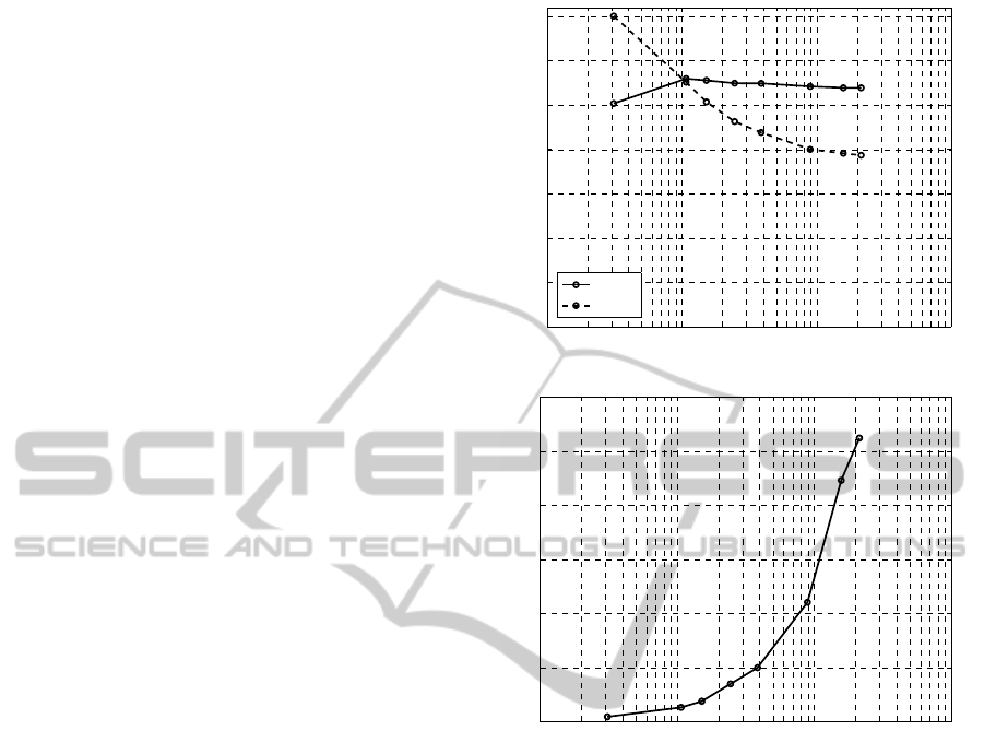
2.5 Grid Convergence

A grid convergence study is conducted using the ON-

ERA M6 wing (NASA, 2008). The ﬂow past the ON-

ERA M6 wing is simulated at various grid resolutions

at Re

∞,c

mac

= 11.72 × 10

, M

∞

= 0.8395 and angle

of attack α = 3.06

◦

, where c

mac

is the mean aerody-

namic chord length. The ﬂow conditions are selected

to match experimental ﬂow conditions of an ONERA

M6 wing experiment 2308 conducted by Schmitt, V.

and F. Charpin (Schmitt and Charpin, 1979), see Sec-

tion 2.6.

The grid convergence study shown in Fig. 4(a)

revealed that 1,576,413 cells are needed for conver-

gence in lift. The drag, however, can still be improved

as evident from Fig. 4(a), where convergence has not

been reached due to limitations in the computational

resources. We proceed, however, with this grid as

the high-ﬁdelity model grid. The overall simulation

time needed for one high-ﬁdelity CFD simulation was

around 223 minutes, as shown in Fig. 4(b), executed

on four Intel-i7-2600 processors in parallel. This exe-

cution time is based on 1000 solver iterations, where

the solver terminated due to the maximum number of

iterations limit.

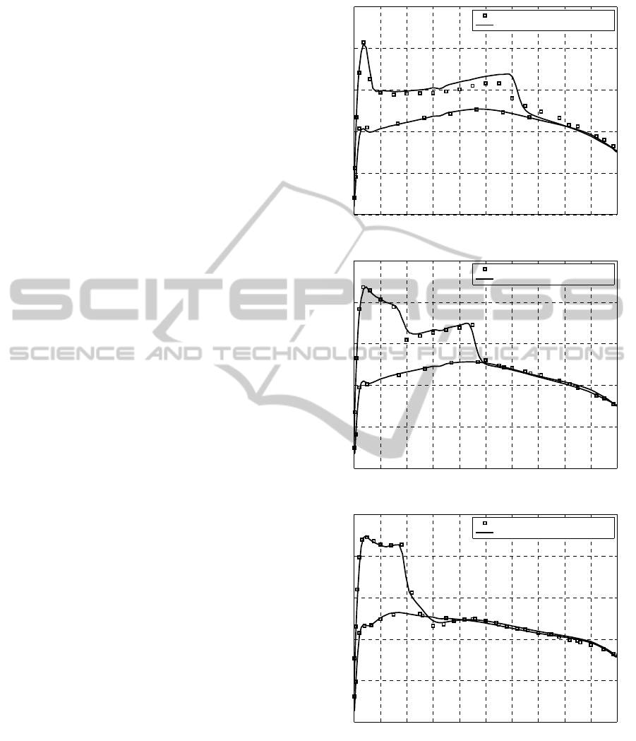
2.6 Model Validation

The ONERA M6 wing is a commonly used CFD val-

idation case for external ﬂows because of its simple

geometry combined with complexities of transonic

ﬂow, i.e., local supersonic ﬂow, shocks, and turbu-

0.05

0.1

0.15

0.2

0.25

0.3

0.35

Number of grid elements

,10 x C

10 x C

(a)

100

150

200

250

300

Number of grid elements

Time [min]

(b)

Figure 4: Grid convergence study using the ONERA M6

wing at Re

∞,c

mac

= 11.72 × 10

, M

∞

= 0.8395 and angle of

attack α = 3.06

◦

. (a) Lift (C

) and drag (C

) coefﬁcients

versus the number of grid elements, and (b) simulation time

versus the number of grid elements.

lent boundary layers with separation. We consider

the ONERA M6 wing as a validation case for the

high-ﬁdelity CFD model. The ONERA M6 wing

is a swept, semi-span wing with no twist and then

symmetrical ONERA D airfoil section (Schmitt and

Charpin, 1979). The numerical coordinates of the

airfoil section at the y/(b/2) = 0 are obtained from

NASA (NASA, 2008). The coordinates indicate that

there is a ﬁnite thickness to the trailing edge. In this

work, we use a zero trailing edge thickness. The air-

foil coordinates are linearly scaled near the trailing

edge so that the trailing edge thickness is zero. We

use experimental data from a ONERA M6 wing wind

tunnel experiment 2308 conducted by Schmitt, V. and

F. Charpin (Schmitt and Charpin, 1979). The solver is

conﬁgured to match the experimental ﬂow conditions

which are Re

∞,c

mac

= 11.72 × 10

, M

∞

= 0.8395, an-

gle of attack α = 3.06

◦

, pressure p

∞

= 80507.2Pa and

SIMULTECH 2012 - 2nd International Conference on Simulation and Modeling Methodologies, Technologies and

Applications

492

temperature T

∞

= 255.6K.

The available experimental data obtained by

Schmitt and Charpin, consists of pressure distribu-

tions (C

) at seven cross-sections along the span,

namely, y/(b/2) = 0.2, 0.44, 0.65, 0.8, 0.9, 0.95, 0.99.

The CFD simulation results are shown for y/(b/2) =

0.2, 0.65, 0.95, in Fig. 5. Inspecting the results, we

see that the correlation between the CFD simulation

and experimental data is excellent.

3 OPTIMIZATION WITH SPACE

MAPPING

In this paper, the wing design is carried out in a com-

putationally efﬁcient manner by exploiting the space

mapping (SM) methodology (Bandler et al., 2004).

Space mapping replaces the direct optimization of an

expensive (high-ﬁdelity or ﬁne) airfoil model f ob-

tained through high-ﬁdelity CFD simulation, by an it-

erative updating and re-optimization of a cheaper sur-

rogate model s. The key component of SM is the

physics-based low-ﬁdelity (or coarse) model c that

embeds certain knowledge about the system under

consideration and allows us to construct a reliable sur-

rogate using a limited amount of high-ﬁdelity model

data. Here, the low-ﬁdelity model is evaluated using

the same CFD solver as the high-ﬁdelity one, so that

both models share the same knowledge of the wing

performance.

3.1 Optimization Problem

The simulation-driven design can be generally formu-

lated as a nonlinear minimization problem

∗

= arg min

H ( f (x)), (1)

where x is a vector of design parameters, f the high-

ﬁdelity model to be minimized at x and H is the ob-

jective function. x

∗

is the optimum design vector.

The high-ﬁdelity model will represent aerodynamic

forces, lift and drag coefﬁcient, as well as other scalar

responses such as cross-sectional area A of the wing at

interesting location. Area response can be of a vector

form A if one requires multiple area cross-sectional

constraints at various locations on the wing, e.g., the

wing root and the wing tip. The response will have to

form

f (x) = [C

L, f

(x),C

D, f

(x),A

(x)]

, (2)

where C

L, f

and C

D, f

are the lift and drag coefﬁcient

for a three-dimensional wing, respectively, generated

by the high-ﬁdelity model. We are interested in the

0 0.1 0.2 0.3 0.4 0.5 0.6 0.7 0.8 0.9 1

−1.5

−1

−0.5

0.5

x/c

3D Schmitt, V. and F. Charpin Data

3D CFD Simulation

(a) y/(b/2) = 0.2.

0 0.1 0.2 0.3 0.4 0.5 0.6 0.7 0.8 0.9 1

−1.5

−1

−0.5

0.5

x/c

3D Schmitt, V. and F. Charpin Data

3D CFD Simulation

(b) y/(b/2) = 0.65.

0 0.1 0.2 0.3 0.4 0.5 0.6 0.7 0.8 0.9 1

−1.5

−1

−0.5

0.5

x/c

3D Schmitt, V. and F. Charpin Data

3D CFD Simulation

Figure 5: Pressure distributions (C

) at y/(b/2) = (a) 0.2;

(b) 0.65 (c) 0.95 of the ONERA M6 wing at M

∞

= 0.8395

and angle of attack α = 3.06

◦

. The CFD simulation results

are shown with a solid line (-). The wind tunnel experi-

mental data (from Schmitt, V. and F. Charpin (Schmitt and

Charpin, 1979)) is shown with square markers.

Transonic Wing Optimization by Variable-resolution Modeling and Space Mapping

493

maximizing lift case, so the objective function will

take the form of

H ( f (x)) = −C

, (3)

the design constraints denoted as

C ( f (x)) = [c

( f (x)) ,...,c

( f (x))]

. (4)

Maximizing lift will yield two nonlinear design

constraints for drag and area,

( f (x)) = C

D, f

(x) −C

D,max

≤ 0, (5)

( f (x)) = −A

(x) + A

min

≤ 0. (6)

where C

D,max

and A

min

are the maximum allowable

drag and minimum allowable cross-sectional area, re-

spectively.

3.2 Space Mapping Basics

Starting from an initial design x

(0)

, the generic space

mapping algorithm produces a sequence x

(i)

,i =

0,1... of approximate solutions to Eq. (1) as

(i+1)

= arg min



(i)

(x)



, (7)

where

(i)

(x) =

(i)

L,s

(x),C

(i)

D,s

(x),A

(x)

(i)

, (8)

is the surrogate model at iteration i. As previously

described, the accurate high-ﬁdelity CFD model f is

accurate but computationally expensive. Using space

mapping, the surrogate s is a composition of the low-

ﬁdelity CFD model c and a simple linear transforma-

tion to correct the low-ﬁdelity model response (Ban-

dler et al., 2004). The corrected response is denoted

as s(x, p), where p represents a set of model parame-

ters and at iteration i the surrogate is

(i)

(x) = s(x, p). (9)

The SM parameters p are determined through a

parameter extraction (PE) process. In general, this

process is a nonlinear optimization problem where the

objective is to minimize the misalignment of surro-

gate response at some or all previous iteration high-

ﬁdelity model data points (Bandler et al., 2004). The

PE optimization problem can be deﬁned as

(i)

= arg min

∑

k=0

i,k

k f (x

(k)

) − s(x

(k)

,p)k

, (10)

where w

i,k

are weight factors that control how much

impact previous iterations affect the SM parameters.

Popular choices are

i,k

= 1 ∀i,k , (11)

and

i,k



1 k = i

0 otherwise

. (12)

In the ﬁrst case, all previous SM iterations inﬂuence

the parameters; in the second case, the parameters de-

pend only on the most recent SM iteration.

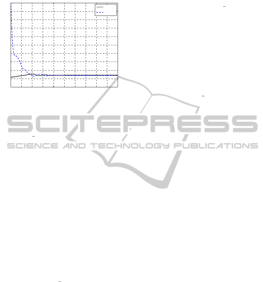
3.3 Low-ﬁdelity CFD Model

The low-ﬁdelity model c is constructed in the same

way as the high-ﬁdelity model f , but with a coarser

grid discretization and with a relaxed convergence cri-

teria - the so called variable-resolution modeling. Re-

ferring back to the grid study made in Section 2.5 and

inspecting Fig. 4(a), we make our selection for the

coarse low-ﬁdelity model. Based on time and accu-

racy with respect of lift and drag, we select the grid

parameters that represent the second point from left,

giving a 107,054 elements. The time taken to eval-

uate the low-ﬁdelity model is 13.2 minutes on four

Intel-i7-2600 processors in parallel. Inspecting fur-

ther the lift and drag convergence plot for the low-

ﬁdelity model in Fig. 6, we note that the solution

has converged after 400-500 iterations. The maxi-

mum number of iterations for the low-ﬁdelity model

is therefore set to 500 iterations. This reduces the

overall simulation time to 6.6 minutes. The ratio of

simulation times of the high- and low- ﬁdelity model

in this case is high/low = 223/6.6 u 34. This is based

on the solver uses all 500 iterations in the low-ﬁdelity

model to obtain a solution.

The low-ﬁdelity CFD model c turns out to be very

noisy. In order to alleviate the problem, a second or-

der polynomial approximation model is constructed

(Koziel et al., 2011) using N

= 50 training points

sampled using latin hypercube sampling (LHS) (For-

rester and Keane, 2009) using the low-ﬁdelity CFD

model. The polynomial approximation model is de-

ﬁned as

c(x) = c

+ c

x + x

x, (13)

where c

= [c

1.1

1.2

1.3

]

and c

= [c

2.i j

]

i, j=1,2,3

The coefﬁcients c

, c

are found by solving a lin-

ear regression problem

c(x

) = c(x

), (14)

SIMULTECH 2012 - 2nd International Conference on Simulation and Modeling Methodologies, Technologies and

Applications

494

100 200 300 400 500 600 700 800 900 1000

0.2

0.4

0.6

0.8

1.2

1.4

1.6

1.8

,10 x C

Iterations

10 x C

Figure 6: Lift and drag coefﬁcient convergence plot for the

low-ﬁdelity model obtained in the grid convergence study

using the ONERA M6 wing at Mach number M

∞

= 0.8395

and angle of attack α = 3.06

◦

where k = 1, . . .,N

. The resulting second order poly-

nomial model c has nice analytical properties, such as

smoothness and convexity.

3.4 Surrogate Model Construction

As mentioned above, the SM surrogate model s is

a composition of the low-ﬁdelity CFD model c and

corrections or linear transformations where the model

parameters p are extracted using one of the PE pro-

cesses described above. The parameter extraction and

the surrogate optimization create a certain overhead

on the whole process and this overhead can be up to

80-90 % of the computational cost. This is due to the

fact that the physics-based low-ﬁdelity models are in

general relatively expensive to evaluate compared to

the functional-based ones. Despite this, SM may be

beneﬁcial (Zhu et al., 2007).

To alleviate this problem, the output SM with both

multiplicative and additive response correction is ex-

ploited here with the surrogate model parameters ex-

tracted analytically. We use the following formulation

(i)

(x) = A

(i)

◦ c(x) + D

(i)

+ q

(i)

(15)

(i)

(x) =

(i)

L,c

(x) + d

(i)

+ q

(i)

D,c

(x) + d

(i)

+ q

(i)

, A

(x)

(16)

where ◦ is a component-wise multiplication. No map-

ping is needed for the area A

(x) where, A

(x) =

(x) ∀x since low- and high-ﬁdelity model repre-

sent the same geometry. Parameters A

(i)

and D

(i)

are

obtained using

(i)

= argmin

A,D

∑

k=0

k f



(k)



− A ◦ c



(k)



+ Dk

(17)

where w

i,k

= 1, i.e., all the previous iteration points

are used to improve globally the response of the

low-ﬁdelity model. The additive term q

(i)

is de-

ﬁned such that is ensures a perfect match between the

surrogate and the high-ﬁdelity model at design x

(i)

namely f



(i)



= s



(i)



or a zero-order consistency

(Alexandrov and Lewis, 2001). We can write the ad-

ditive term as

(i)

= f



(i)



−

(i)

◦ c(x

(i)

) + D

(i)

. (18)

Since analytical solution exists for A

(i)

and

(i)

there is no need for non-linear optimization for

solving Eq. (10) to obtain the parameters. We can

obtain A

(i)

and D

(i)

by solving

(i)





−1

, (19)

(i)





−1

, (20)

where



L,c

(0)

) C

L,c

(1)

) ... C

L,c

(i)

)

1 1 ... 1



(21)



L, f

(0)

) C

L, f

(1)

) ... C

L, f

(i)

)

1 1 ... 1



(22)



D,c

(0)

) C

D,c

(1)

) ... C

D,c

(i)

)

1 1 ... 1



(23)



D, f

(0)

) C

D, f

(1)

) ... C

D, f

(i)

)

1 1 ... 1



(24)

which are the least-square optimal solutions to the lin-

ear regression problems

(i)

+ d

(i)

= F

, (25)

(i)

+ d

(i)

= F

. (26)

Note that C

and C

are non-singular for

i > 1 and assuming that x

(k)

6= x

(i)

for k 6= i. For i =

1 only the multiplicative SM correction with A

(i)

used.

Transonic Wing Optimization by Variable-resolution Modeling and Space Mapping

495

3.5 Optimization Algorithm

Here, we formulate the optimization algorithm ex-

ploiting the SM based surrogate and a trust-region

convergence safeguard (Forrester and Keane, 2009).

The trust-region parameter λ is updated after each it-

eration. This algorithm will be used in applications

presented in this thesis. The optimization algorithm

is as follows:

1. Set i = 0; Select λ, the trust region radius; Eval-

uate the high-ﬁdelity model at the initial solution,

f (x

(0)

);

2. Using data from the low-ﬁdelity model c, and f

at x

(k)

,k = 0, 1, . ..,i, setup the SM surrogate s

(i)

;

Perform PE;

3. Optimize s

(i)

to obtain x

(i+1)

;

4. Evaluate f (x

(i+1)

);

5. If H( f (x

(i+1)

)) < H( f (x

(i)

)), accept x

(i+1)

; Oth-

erwise set x

(i+1)

= x

(i)

;

6. Update λ;

7. Set i = i + 1;

8. If the termination condition is not satisﬁed, go to

2, else proceed;

9. End; Return x

(i)

as the optimum solution.

The termination condition is set to kx

(i)

− x

(i−1)

k <

−3

4 NUMERICAL EXAMPLES

In this section, we apply the proposed optimization

algorithm to the lift maximization of a rectangular

wing at transonic conditions. The direct solution

of the original problem in Eq. (1) has not been at-

tempted due to the heavy computational cost of the

high-ﬁdelity model. We formulate the problem and

describe the setup. Then, we present the results of

numerical optimization.

4.1 Setup

The wing is unswept and untwisted and is constructed

by two NACA 4 digit airfoils, located at the root and

tip, as described in Fig. 1. The root airfoil is ﬁxed

to be NACA 2412. The tip airfoil is to be designed.

The initial design x

(0)

for the wing tip is chosen at

random at the start of each optimization run. The

normalized semi-wingspan is set as twice the wing

chord length c as (b/2) = 2c. All other wing param-

eters are kept ﬁxed. The design vector can be written

as x = [m, p,t/c]

, where the variables represent the

wing tip NACA 4 digit airfoil parameters.

The objective is to maximize the lift coefﬁcient

L, f

subject to constraints on the drag coefﬁcient

D, f

≤ C

D,max

= 0.03 and the wing tip normalized

cross-sectional area A ≥ A

min

= 0.01. The side con-

straints on the design variables are 0.02 ≤ m ≤ 0.03,

0.7 ≤ p ≤ 0.9 and 0.06 ≤ t/c ≤ 0.08.

4.2 Results

Two optimization runs were performed, denoted as

Run 1 and Run 2. The numerical results are given

in Table 1, and the initial and optimized airfoil cross-

sections are shown in Fig. 7(a) and Fig. 7(b), respec-

tively.

In Run 1, the lift is increased by +10% and the

drag is pushed above its constraint at C

D,max

= 0.03,

where the optimized drag coefﬁcient is C

= 0.0311.

The drag constraint is violated slightly, or by +4%,

which is within the 5% constraint tolerance band. The

lift-to-drag ratio is decreased by -14%. The proposed

method requires less than 10 high-ﬁdelity model eval-

uations, where 50 low-ﬁdelity model evaluations are

used to create the approximation model and 8 high-

ﬁdelity model evaluations for each design iteration. It

is evident that the optimized wing tip airfoil is thicker

as the normalized cross-sectional area is increased by

+26%, and the increased drag can be related to the in-

crement in area. No change is in the camber m, but

the location of the maximum camber p has moved

slightly aft.

The initial design for Run 2 violates the drag con-

straint. The proposed method is, however, able to

push the drag to its constraint limit where the opti-

mized drag coefﬁcient is slightly violated, by +2%).

While the drag is decreased by -11%, the lift is main-

tained and only drops by -1%. As a result, the lift-

to-drag ratio is increased by +11%. The proposed

method requires less than 9 high-ﬁdelity model eval-

uations (50 low-ﬁdelity model evaluations used to

create the approximation model and 7 high-ﬁdelity

model evaluations). The optimized wing tip airfoil is

thinner than the initial design (the normalized cross-

sectional area is reduced by -20%). Little changes are

made to the camber m and the maximum camber lo-

cation p.

Comparing runs 1 and 2, we note that although

starting from different initial designs the optimized

designs show similarities in two of three design vari-

ables, the maximum camber m and maximum camber

location p. The third, the airfoil thickness t/c differs

by approximately 2%. The shock on the mid wing has

been moved aft on both the upper and the lower sur-

SIMULTECH 2012 - 2nd International Conference on Simulation and Modeling Methodologies, Technologies and

Applications

496

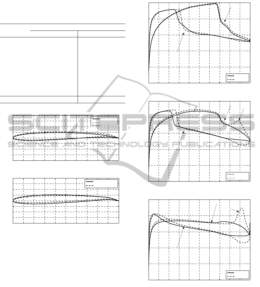
Table 1: Numerical comparison of Run 1 and Run 2, initial

and optimized designs. The ratio of the high-ﬁdelity model

evaluation time to the low-ﬁdelity is 34.

Initial Optimized

Variable Run 1 Run 2 Run 1 Run 2

m 0.0200 0.0259 0.0200 0.0232

p 0.7000 0.8531 0.8725 0.8550

t/c 0.0628 0.0750 0.0793 0.0600

0.2759 0.3426 0.3047 0.3388

0.0241 0.0344 0.0311 0.0307

11.4481 9.9593 9.7974 11.0358

A 0.0422 0.0505 0.0534 0.0404

- - 50 50

- - 8 7

Total Cost - - < 10 < 9

0 0.1 0.2 0.3 0.4 0.5 0.6 0.7 0.8 0.9 1

−0.2

−0.15

−0.1

−0.05

0.05

0.1

0.15

0.2

x/c

z/c

Run 1 Initial

Run 2 Initial

(a) Initial.

0 0.1 0.2 0.3 0.4 0.5 0.6 0.7 0.8 0.9 1

−0.2

−0.15

−0.1

−0.05

0.05

0.1

0.15

0.2

x/c

z/c

Run 1 Optimized

Run 2 Optimized

(b) Optimized.

Figure 7: A comparison of Run 1 and Run 2, initial and

optimized designs. (a) Initial design comparison, and (b)

Optimized comparison. Run 1 is shown with a solid lines

(–), and Run 2 with dashed lines (- -).

faces. Also, a second shock as formed near the tip on

the upper surface. This causes the drag rise, as well

as an increase in lift since the pressure distribution has

opened up, as can be seen from Fig. 8.

5 CONCLUSIONS

A robust and efﬁcient aerodynamic design optimiza-

tion methodology for wings using high-ﬁdelity CFD

models has been presented. Our approach exploits

a cheap surrogate model to obtain an approximate

optimum design of an expensive high-ﬁdelity CFD

0 0.1 0.2 0.3 0.4 0.5 0.6 0.7 0.8 0.9 1

−1

−0.5

0.5

1.5

x/c

Inital

Optimized

Upper Surface

Lower Surface

(a) y/(b/2) = 0.2.

0 0.1 0.2 0.3 0.4 0.5 0.6 0.7 0.8 0.9 1

−1

−0.5

0.5

1.5

x/c

Inital

Optimized

Upper Surface

Lower Surface

Shock

(b) y/(b/2) = 0.65.

0 0.1 0.2 0.3 0.4 0.5 0.6 0.7 0.8 0.9 1

−1

−0.5

0.5

1.5

x/c

Inital

Optimized

Upper Surface

Lower Surface

Shock

Figure 8: Pressure distributions of the initial and optimized

design of Run 1 at y/(b/2) = (a) 0.2, (b) 0.65, and (c) 0.95,

where M

∞

= 0.8395 and angle of attack α = 3.06

◦

. Initial

design is shown with a solid line (–) and the optimum design

with a dashed line (- -).

model. The surrogate model is constructed using

a corrected second-order polynomial approximation

model derived from low-ﬁdelity CFD model data.

The correction is performed using the output space

Transonic Wing Optimization by Variable-resolution Modeling and Space Mapping

497

mapping technique. The space mapping correction is

applied both to the objectives and the constraints, en-

suring zero-order consistency and a perfect alignment

between the surrogate and the high-ﬁdelity model. To

our knowledge, this is the ﬁrst application of the space

mapping methodology used in conjunction with low-

ﬁdelity approximation models in aerodynamic shape

optimization. The proposed approach performs well

and optimized designs are obtained using only a few

high-ﬁdelity model evaluations.

ACKNOWLEDGEMENTS

This work was funded by The Icelandic Research

Fund for Graduate Students, grant ID: 110395-0061.

REFERENCES

Abbott, I. and Von Doenhoff, A. (1959). Theory of wing

sections: including a summary of airfoil data. Dover.

Alexandrov, N. and Lewis, R. (2001). An overview of ﬁrst-

order model management for engineering optimiza-

tion. Optimization and Engineering, 2(4):413–430.

ANSYS (2010). ANSYS FLUENT Theory Guide. AN-

SYS, Southpointe 275 Thecnology Drive Canonburg

PA 15317, release 13.0 edition.

Bandler, J., Cheng, Q., Dakroury, S., Mohamed, A., Bakr,

M., Madsen, K., and Sondergaard, J. (2004). Space

mapping: the state of the art. Microwave Theory and

Techniques, IEEE Transactions on, 52(1):337–361.

Echeverria, D. and Hemker, P. (2005). Space mapping and

defect correction. Computational Methods in Applied

Mathematics, 5(2):107–136.

Forrester, A. and Keane, A. (2009). Recent advances in

surrogate-based optimization. Progress in Aerospace

Sciences, 45(1-3):50–79.

Haikin, S. (1998). Neural Networks: A Comprehensive

Foundation. Prentice Hall.

Journel, A. and Huijbregts, C. (1978). Mining geostatistics.

Academic press.

Koziel, S., Cheng, Q., and Bandler, J. (2008). Space map-

ping. Microwave Magazine, IEEE, 9(6):105–122.

Koziel, S., Ciaurri, D. E., and Leifsson, L. (2011).

Surrogate-based methods. In Computational opti-

mization and applications in engineering and indus-

try, volume 359. Springer.

Koziel, S. and Leifsson, L. (2012). Knowlegde-based air-

foil shape optimization using space mapping. In 30th

AIAA Applied Aerodynamics Conference.

Leifsson, L. and Koziel, S. (2011a). Airfoil shape opti-

mization using variable-ﬁdelity modeling and shape-

preserving response prediction. In Comp. Opt., Meth-

ods and Algorithms, volume 356. Springer.

Leifsson, L. and Koziel, S. (2011b). Variable-ﬁdelity aero-

dynamic shape optimization. In Comp. Opt., Methods

and Algorithms, volume 356. Springer.

Minsky, M. and Papert, S. (1969). Perceptrons: An intro-

duction to computational geometry. The MIT Press,

Cambridge, MA.

NASA (2008). Onera-m6-wing validation case. In

http://www.grc.nasa.gov.

O’Hagan, A. and Kingman, J. (1978). Curve ﬁtting and

optimal design for prediction. Journal of the Royal

Statistical Society. Series B (Methodological).

Queipo, N., Haftka, R., Shyy, W., Goel, T., Vaidyanathan,

R., and Kevin Tucker, P. (2005). Surrogate-based anal-

ysis and optimization. Progress in Aerospace Sci-

ences, 41(1):1–28.

Raymer, D. (2006). Aircraft design: a conceptual approach.

American Institute of Aeronautics and Astronautics.

Robinson, T., Willcox, K., Eldred, M., and Haimes,

R. (2006). Multiﬁdelity optimization for variable-

complexity design. In Proceedings of the 11th

AIAA/ISSMO Multidisciplinary Analysis and Opti-

mization Conference, Portsmouth, VA.

Schmitt, V. and Charpin, F. (1979). Pressure distributions

on the onera-m6-wing at transonic mach numbers. Ex-

perimental Data Base for Computer Program Assess-

ment, Report of the Fluid Dynamics Panel Working

Group 04, AGARD AR 138, May 1979.

Simpson, T., Poplinski, J., Koch, P., and Allen, J. (July

2001). Metamodels for computer-based engineering

design: survey and recommendations. Engineering

with computers, 17(2):129–150.

Smola, A. and Sch

olkopf, B. (2004). A tutorial on sup-

port vector regression. Statistics and computing,

14(3):199–222.

Søndergaard, J. (2003). Optimization using surrogate mod-

els by the space mapping technique. PhD thesis, PhD.

Thesis, Technical University of Denmark, Informatics

and mathematical modelling.

Tannehill, J., Anderson, D., and Pletcher, R. (1997). Com-

putational ﬂuid mechanics and heat transfer. Taylor

& Francis Group.

Wild, S., Regis, R., and Shoemaker, C. (2008). Orbit:

Optimization by radial basis function interpolation in

trust-regions. SIAM Journal on Scientiﬁc Computing,

30(6):3197–3219.

Zhu, J., Bandler, J., Nikolova, N., and Koziel, S. (2007).

Antenna optimization through space mapping. An-

tennas and Propagation, IEEE Transactions on,

55(3):651–658.

SIMULTECH 2012 - 2nd International Conference on Simulation and Modeling Methodologies, Technologies and

Applications

498