
Simple Fuzzy Logic Models to Estimate the Global Temperature
Change Due to GHG Emissions
Carlos Gay García
1
, Oscar Sánchez Meneses
1
, Benjamín Martínez-López
1
, Àngela Nebot
2
and Francisco Estrada
1
1
Centro de Ciencias de la Atmósfera, Universidad Nacional Autónoma de México, Ciudad Universitaria, D.F., Mexico
2
Grupo de Investigación Soft Computing, Universitat Politècnica de Catalunya, Barcelona, Spain
Keywords: Fuzzy Inference Models, Greenhouse Gases Future Scenarios, Global Climate Change.
Abstract: Future scenarios (through 2100) developed by the Intergovernmental Panel on Climate Change (IPCC)
indicate a wide range of concentrations of greenhouse gases (GHG) and aerosols, and the corresponding
range of temperatures. These data, allow inferring that higher temperature increases are directly related to
higher emission levels of GHG and to the increase in their atmospheric concentrations. It is evident that
lower temperature increases are related to smaller amounts of emissions and, to lower GHG concentrations.
In this work, simple linguistic rules are extracted from results obtained through the use of simple linear
scenarios of emissions of GHG in the Magicc model. These rules describe the relations between the GHG,
their concentrations, the radiative forcing associated with these concentrations, and the corresponding
temperature changes. These rules are used to build a fuzzy model, which uses concentration values of GHG
as input variables and gives, as output, the temperature increase projected for year 2100. A second fuzzy
model is presented on the temperature increases obtained from the same model but including a second
source of uncertainty: climate sensitivity. Both models are very attractive because their simplicity and
capability to integrate the uncertainties to the input (emissions, sensitivity) and the output (temperature).
1 INTRODUCTION
There is a growing scientific consensus that
increasing emissions of greenhouse gases (GHG) are
changing the Earth's climate. The IPCCs Fourth
Assessment Report (IPCC, 2007) states that
warming of the climate system is unequivocal and
notes that eleven of the last twelve years (1995-
2006) rank among the twelve warmest years of
recorded temperatures (since 1850). The projections
of the IPCCs Third Assessment Report (TAR)
(IPCC, 2001) regarding future global temperature
change ranged from 1.4 to 5.8 °C. More recently, the
projections indicate that temperatures would be in a
range spanning from 1.1 to 4 °C, but that
temperatures increases of more than 6 °C could not
be ruled out (IPCC; 2007). This wide range of
values reflects the uncertainty in the production of
accurate projections of future climate change due to
different potential pathways of GHG emissions.
There are other sources of the uncertainty preventing
us from obtaining better precision. One of them is
related to the computer models used to project future
climate change. The global climate is a highly
complex system due to many physical, chemical,
and biological processes that take place among its
subsystems within a wide range of space and time
scales.
Global circulation models (GCM) based on the
fundamental laws of physics try to incorporate those
known processes considered to constitute the climate
system and are used for predicting its response to
increases in GHG (IPCC, 2001). However, they are
not perfect representations of reality because they do
not include some important physical processes (e.g.
ocean eddies, gravity waves, atmospheric
convection, clouds and small-scale turbulence)
which are too small or fast to be explicitly modeled.
The net impact of these small scale physical
processes is included in the model by means of
parameterizations (Schmidt, 2007). In addition,
more complex models imply a large number of
parameterized processes and different models use
different parameterizations. Thus, different models,
using the same forcing produce different results.
One of the main sources of uncertainty is,
518
Gay García C., Sánchez Meneses O., Martínez-López B., Nebot À. and Estrada F..
Simple Fuzzy Logic Models to Estimate the Global Temperature Change Due to GHG Emissions.
DOI: 10.5220/0004164905180526
In Proceedings of the 2nd International Conference on Simulation and Modeling Methodologies, Technologies and Applications (MSCCEC-2012), pages
518-526
ISBN: 978-989-8565-20-4
Copyright
c
2012 SCITEPRESS (Science and Technology Publications, Lda.)

however, the different potential pathways for
anthropogenic GHG emissions, which are used to
drive the climate models. Future emissions depend
on numerous driving forces, including population
growth, economic development, energy supply and
use, land-use patterns, and a variety of other human
activities (Special Report on Emissions Scenarios,
SRES). Future temperature scenarios have been
obtained with the emission profiles corresponding to
the four principal SRES families (A1, A2, B1, and
B2) (Nakicenovic et al., 2000). From the point of
view of a policy-maker, the results of the 3rd and 4th
IPCC’s assessments regarding the projection of
global or regional temperature increases are difficult
to interpret due to the wide range of the estimated
warming. Nevertheless this is an aspect of
uncertainty that scientists and ultimately policy-
makers have to deal with. Furthermore, most of the
available methodologies that have been proposed for
supporting decision-making under uncertainty do not
take into account the nature of climate change’s
uncertainty and are based on classic statistical theory
that might not be adequate. Climate change’s
uncertainty is predominately epistemic and,
therefore, it is critical to produce or adapt
methodologies that are suitable to deal with it and
that can produce policy-useful information. The lack
of such methodologies is noticeable in the IPCC’s
AR4 Contribution of the Working Group I, where
the proposed best estimates, likely ranges and
probabilistic scenarios are produced using
statistically questionable devices (Gay and Estrada,
2009).
Two main strategies have been proposed for
dealing with uncertainty: trying to reduce it by
improving the science of climate change a feat tried
in the AR4 of the IPCC, and integrating it into the
decision-making processes (Schneider, 2003). There
are clear limitations regarding how much of the
uncertainty can be reduced by improving the state of
knowledge of the climate system, since there
remains the uncertainty about the emissions which is
more a result of political and economic decisions
that do not necessarily obey natural laws.
Therefore, we propose that the modern view of
climate modelling and decision-making should
become more tolerant to uncertainty because it is a
feature of the real world (Klir and Elias, 2002).
Choosing a modelling approach that includes
uncertainty from the start tends to reduce its
complexity and promotes a better understanding of
the model itself and of its results. Science and
decision-making have always had to deal with
uncertainty and various methods and even branches
of science, such as Probability, have been developed
for this matter (Jaynes, 1957). Important efforts have
been made for developing approaches that can
integrate subjective and partial information, being
the most successful ones Bayesian and maximum
entropy methods and more recently, fuzzy set theory
where the concept of objects that have not precise
boundaries was introduced (Zadeh, 1965). Fuzzy
logic provides a meaningful and powerful
representation of uncertainties and is able to express
efficiently the vague concepts of natural language
(Zadeh, 1965). These characteristics could make it a
very powerful and efficient tool for policy makers
due to the fact that the models are based on
linguistic rules that could be easily understood.
In this paper two fuzzy logic models are
proposed for the global temperature changes (in the
year 2100) that are expected to occur in this century.
The first model incorporates the uncertainties related
to the wide range of emission scenarios and
illustrates in a simple manner the importance of the
emissions in determining future temperatures. The
second incorporates the uncertainty due to climate
sensitivity that pretends to emulate the diversity in
modelling approaches. Both models are built using
the Magicc (Wigley, 2008) model and Zadeh´s
extension principle for functions where the
independent variable belongs to a fuzzy set. Magicc
is capable of emulating the behaviour of complex
GCMs using a relative simple one dimensional
model that incorporates different processes e.g.
carbon cycle, earth-ocean diffusivity, multiple gases
and climate sensitivity. In our second case we intend
to illustrate the combined effects of two sources of
uncertainty: emissions and model sensitivity. It is
clear that we are leaving out of this paper other
important sources of uncertainty whose contribution
would be interesting to explore. The GCMs are,
from our point of view, useful and very valuable
tools when it is intended to study specific aspects or
details of the global temperature change.
Nevertheless, when the goal is to study and to test
global warming policies, simpler models much
easier to understand become very attractive. Fuzzy
models can perform this task very efficiently.
2 FUZZY LOGIC MODEL
OBTAINED FROM IPCC DATA
The Fourth Assessment Report of the IPCC shows
estimates of emissions, concentrations, forcing and
temperatures through 2100 (IPCC, 2007). Although
there are relationships among these variables, as
SimpleFuzzyLogicModelstoEstimatetheGlobalTemperatureChangeDuetoGHGEmissions
519
those reflected in the figure 1 (upper panel), it would
be useful to find a way to relate emissions directly
with increases of temperature. A more physical
relation is established between concentrations and
temperature because the latter depends almost
directly upon the former through the forcing terms.
Concentrations are obtained integrating over time
the emissions minus the sinks of the GHGs. One
way of relating directly emissions and temperature,
could be achieved if the emission trajectories were
linear and non-intersecting as illustrated in figure 1
(upper panel). Here, we perform this task by means
of a fuzzy model, which is based on the Magicc
model (Wigley, 2008) and Zadeh´s extension
principle (see Appendix).
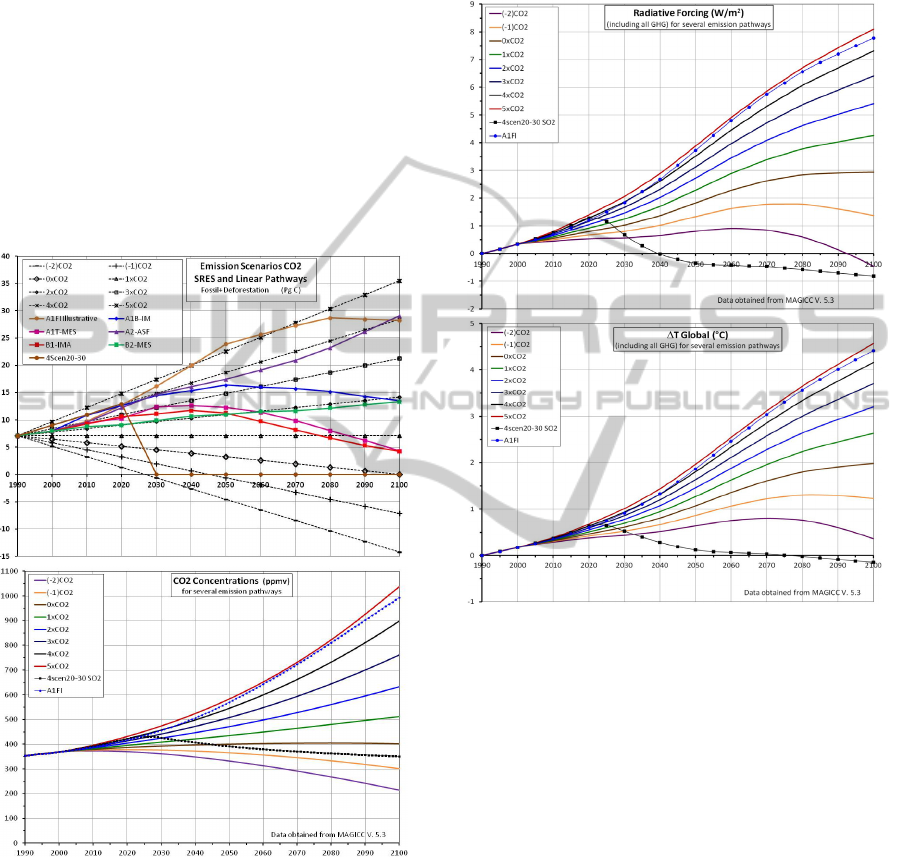
Figure 1: Upper panel: Emissions scenarios CO2,
Illustrative SRES and Linear Pathways. (-2) CO2 means -
2 times the emission (fossil + deforestation) of CO2 of
1990 by 2100 and so for -1, 0, 1, to 5 CO2. All the linear
pathways contain the emission of non CO2 GHG as those
of the A1FI. 4scen20-30 scenario follows the pathway of
4xCO2 but at 2030 all gases drop to 0 emissions or
minimum value in CH4, N2O and SO2 cases. Lower
panel: CO2 Concentrations for linear emission pathways,
4scen20-30 SO2 and A1FI are shown for reference. Data
calculated using Magicc V. 5.3.
Using as input for the Magicc model the
emissions shown in the previous figure we calculate
the resulting concentrations (figure 1 lower panel);
forcings (figure 2 upper panel) and global mean
temperature increments (figure 2 lower panel).
Figure 2: Upper panel: Radiative forcings (all GHG
included) for linear emission pathways and A1FI SRES
illustrative, the 4scen20-30 SO2 only include SO2. Lower
panel: Global temperature increments for linear emission
pathways, 4scen20-30 SO2 and A1FI as calculated using
Magicc V. 5.3.
The set of emissions shown in figure 1 (upper
panel) has been simplified to linear functions of time
that reach by the year 2100 values from minus two
times to 5 times the emissions of 1990. The
trajectories labelled 5CO2 and (-2) CO2 contain the
trajectories of the SRES. We observe that the
concentrations corresponding to the 5CO2 and the
A1FI trajectories, by year 2100 are very close. The
choice of linear pathways allows us to associate
emissions to concentrations to forcings and
temperatures in a very simple manner. We can say
than any trajectory of emissions contained within
two of the linear ones will correspond, at any time
with a temperature that falls within the interval
delimited by the temperatures corresponding to the
linear trajectories. This is illustrated for the A1FI
SIMULTECH2012-2ndInternationalConferenceonSimulationandModelingMethodologies,Technologiesand
Applications
520

trajectory, in figure 2 (lower panel) that falls within
the temperatures of the 5CO2 and 4CO2 trajectories.
We decided to find emission paths that would lead to
temperatures of two degrees or less by the year
2100, this led us to the -2CO2, -1CO2 and 0CO2.
The latter is a trajectory of constant emissions equal
to the emissions in 1990 that gives us a temperature
of two degrees by year 2100.
From the linear representation, it is easily
deduced that very high emissions correspond to very
large concentrations, forcings and large increases of
temperature. It is also possible to say that large
concentrations correspond to large temperature
increases etc. This last statement is very important
because in determining the temperature the climate
models directly use the concentrations which are the
time integral of sources and sinks of the green house
gases (GHG). Therefore the detailed history of the
emissions is lost. Nevertheless the statement, to
large concentrations correspond large temperature
increases still holds. These simple observations
allows us to formulate a fuzzy model, based on
linguistic rules of the IF-THEN form, which can be
used to estimate increases of temperature within
particular uncertainty intervals. Fuzzy logic provides
a meaningful and powerful representation of
measurement of uncertainties, and it is able to
represent efficiently the vague concepts of natural
language, of which the climate science is plagued.
Therefore, it could be a very useful tool for decision
makers. The basic concepts of fuzzy logic are
presented in Appendix.
The first fuzzy model one input one output
defined for the global temperature change is
(quantities between parenthesis were used with
Zadeh’s principle to generate the fuzzy model, the
number 1 means the membership value (μ) of the
input variables used in formulating the fuzzy
model):
1. If (concentration is very low
(about -2CO2)) then (deltaT is very low
(1)
2. If (concentration is low (about -
1CO2)) then (deltaT is low (1)
3. If (concentration is medium-low
(about 0CO2) then (deltaT is medium-low
(1)
4. If (concentration is medium
(about 1CO2)) then (deltaT is medium
(1)
5. If (concentration is medium-high
(about 2CO2)) then (deltaT is medium-
high (1)
6. If (concentration is high (about
3CO2)) then (deltaT is high (1)
7. If (concentration is very high
(about 4CO2)) then (deltaT is very high
(1)
8. If (concentration is extremely
high (about 5CO2)) then (deltaT is
extremely high (1)
The 8 rules for concentration are based on 8 adjacent
triangular membership functions (the simplest form)
corresponding to linear emission trajectories (-2CO2
to 5CO2). The concentrations were obtained from
Magicc model and cover the entire range (210 to
1045 ppmv). The apex of each membership function
(μ=1) corresponds with the base (μ=0) of the
adjacent one, as we show below:
(μ=0, μ=1, μ=0)
1. -2CO2 (210, 213, 300)
2. -1CO2 (213, 300, 401)
3. 0CO2 (300, 401, 513)
4. 1CO2 (401, 513, 633)
5. 2CO2 (513, 633, 762)
6. 3CO2 (633, 762, 899)
7. 4CO2 (762, 899, 1038)
8. 5CO2 (899, 1038, 1045)
The global temperature changes were obtained
through Zadeh’s extension principle applied to data
from Magicc model.
From the point of view of a policy maker, a
fuzzy model as the one represented by the previous
rules is a very useful tool to study the effect of
different policies on the increases of temperature.
The fuzzy rules model can be evaluated by
means of the fuzzy inference process in such a way
that each possible concentration value is mapped
into an increase of temperature value by means of
the Mamdani’s defuzzification process (see
Appendix). The resulting increases of temperature at
year 2100 for each possible concentration (emission
in the case of our linear model) value (solid line) are
shown in the upper panel of figure 3.
The lower panel illustrates the formulation of the
rules by showing the fuzzy set associated with the
different classes of concentrations, the antecedent of
the fuzzy rule, the IF part and the consequent fuzzy
set temperature, the THEN part. The figure 3 lower
panel also illustrates the uncertainties of one
estimation: If the concentration is of 401 ppmv (it
fires rule number 3) within an uncertainty interval of
(300 to 513 ppmv) 4 then the temperature increment
is 1.95 degrees within an uncertainty interval of
(1.23 to 2.63 deg C) in this case the temperatures
will have uncertainties of one or two times the
intervals defined by the expert or the researcher.
SimpleFuzzyLogicModelstoEstimatetheGlobalTemperatureChangeDuetoGHGEmissions
521
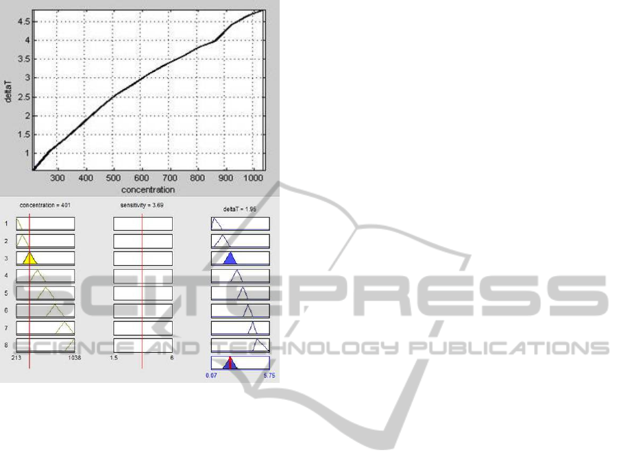
Figure 3: Fuzzy model based on linguistic rules and
Zadeh´s principle. Upper panel: increases of temperature
at year 2100 for each possible concentration (emission in
the case of our linear model) value (solid line). Lower
panel: Fuzzy rules associated with the different classes of
concentrations. (Calculated with MATLAB).
The fuzzy model is simpler and obviously less
computationally expensive than the set of GCM’s
reported by the IPCC. The most important benefit,
however, is its usefulness for policy-makers. For
example, if the required increase of temperature
should be very low or low (-2CO2, -1CO2), then the
policy-maker knows, on the basis of this model, that
concentrations should not exceed the class small.
3 A SIMPLE CLIMATE MODEL
AND ITS CORRESPONDING
FUZZY MODEL
Here, we again use the Magicc model but this time
we introduce a second source of uncertainty, the
climate sensitivity. The purpose is to illustrate the
effects of the combination of two sources of
uncertainty on the resulting temperatures. The
climate model is driven by our linear emission paths.
The relationship between concentrations and
sensitivity and increases of temperature at year 2100
is then used to construct a fuzzy model following the
extension principle of the fuzzy logic approach (see
Appendix).
The set of fuzzy rules obtained in this case is the
following.
1. If (concentration is very very
low) and (sensitivity is low) then
(deltaT is low) (1)
2. If (concentration is very low)
and (sensitivity is low) then (deltaT
is low) (1)
3. If (concentration is very low)
and (sensitivity is high) then (deltaT
is med) (1)
4. If (concentration is medium-low)
and (sensitivity is low) then (deltaT
is low) (1)
5. If (concentration is medium-low)
and (sensitivity is high) then (deltaT
is high) (1)
6. If (concentration is medium) and
(sensitivity is low) then (deltaT is
med) (1)
7. If (concentration is medium) and
(sensitivity is high) then (deltaT is
high) (1)
8. If (concentration is medium-high)
and (sensitivity is low) then (deltaT
is med) (1)
9. If (concentration is medium-high)
and (sensitivity is high) then (deltaT
is high) (1)
10. If (concentration is high) and
(sensitivity is low) then (deltaT is
med) (1)
11. If (concentration is high) and
(sensitivity is high) then (deltaT is
high) (1)
12. If (concentration is medium-low)
and (sensitivity is med) then (deltaT
is med) (1)
Note that we have used the same nomenclature as
before and the very high and extremely high
concentrations are not considered.
And the fuzzy sets for the temperature and
sensitivity are shown in figure 4. We used this figure
to build the rule above in combination with 6 fuzzy
sets for concentration similar to those from our first
model described in section 2:
(μ=0, μ=1, μ=0)
1. -2CO2 (100, 213, 300)
2. -1CO2 (213, 300, 401)
3. 0CO2 (300, 401, 513)
4. 1CO2 (401, 513, 633)
5. 2CO2 (513, 633, 762)
6. 3CO2 (633, 762, 899)
SIMULTECH2012-2ndInternationalConferenceonSimulationandModelingMethodologies,Technologiesand
Applications
522
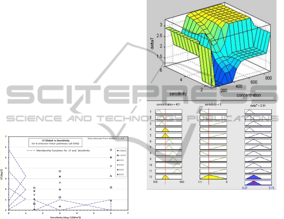
For sensitivity we built 3 triangular fuzzy sets
corresponding to sensitivity values of 1.5, 3 and 6
deg C/W/m2, showed below:
(μ=0, μ=1, μ=0)
1. 1.5 (low) (1.5, 1.5, 3.0)
2. 3.0 (medium) (1.5, 3.0, 6.0)
3. 4.5 (high) (3.0, 6.0, 6.0)
Similarly, for global temperature change we have 3
triangular fuzzy sets built with data obtained from
Magicc model and Zadeh’s extension principle for
each sensitivity value; the apex of each fuzzy set is
the value of global temperature change for the 0CO2
linear emission path according to the value of
sensitivity, the base of the fuzzy sets range from -
2CO2 to 3CO2 (assuming global temperature
changes below 6 deg C) for each sensitivity value
(see figure 4):
( μ=0, μ=1, μ=0)
1. Low (0.07, 1.07, 2.13)
2. Medium (0.36, 1.98, 3.70)
3. High (0.92, 3.27, 5.75)
Figure 4: ΔT Global and sensitivity fuzzy sets for six
linear emission pathways at 2100. The dashed lines show
the membership functions.
The Mamdani’s fuzzy inference method is used
also here as the defuzzification method to compute
the increase of temperature values. The results are
shown in figure 5. The upper panel of figure 5 shows
the surface resulting from the defuzzification
process. The lower panel illustrates again that for the
case of a concentration of 401 ppmv and a
sensitivity of 3 (medium sensitivity) the temperature
is about 2 degrees within an uncertainty interval of
(0.36 to 3.70 deg C) where the membership value is
different from 0. When we compare our previous
result with this one we find that the answers are very
close in fact the fall within the uncertainty intervals
of both. The uncertainty of concentrations and
sensitivity are respectively (300 to 513 ppmv) and
(1.5 to 6 deg C/W/m2). The result is to be expected
since in our first experiment we used the Magicc
model with default value for the sensitivity and this
turns to be of 3.
Figure 5: Fuzzy model for concentrations and sensitivities.
Upper panel: ΔT surface. Lower panel: Fuzzy rules.
(Calculated with MATLAB).
4 DISCUSSION AND
CONCLUSIONS
In this work, simple linguistic fuzzy rules relating
concentrations and increases of temperatures are
extracted from the application of the Magicc model.
The fuzzy model uses concentration values of GHG
as input variable and gives, as output, the increase of
temperature projected at year 2100. A second fuzzy
model based on linguistic rules is developed based
on the same Magicc climate model introducing a
second source of uncertainty coming from the
different sensitivities used by the Magicc to emulate
more complicated GCMs used in the IPCC reports.
These kind of fuzzy models are very useful due to
their simplicity and to the fact that include the
SimpleFuzzyLogicModelstoEstimatetheGlobalTemperatureChangeDuetoGHGEmissions
523
uncertainties associated to the input and output
variables. Simple models that, however, could
contain all the information that is necessary for
policy makers, these characteristics of the fuzzy
models allow not only the understanding of the
problem but also the discussion of the possible
options available to them. For example going back
to the question of stabilizing global temperatures at
about 2 degrees or less, we can see the fuzziness of
the proposition; we could estate that we should stay
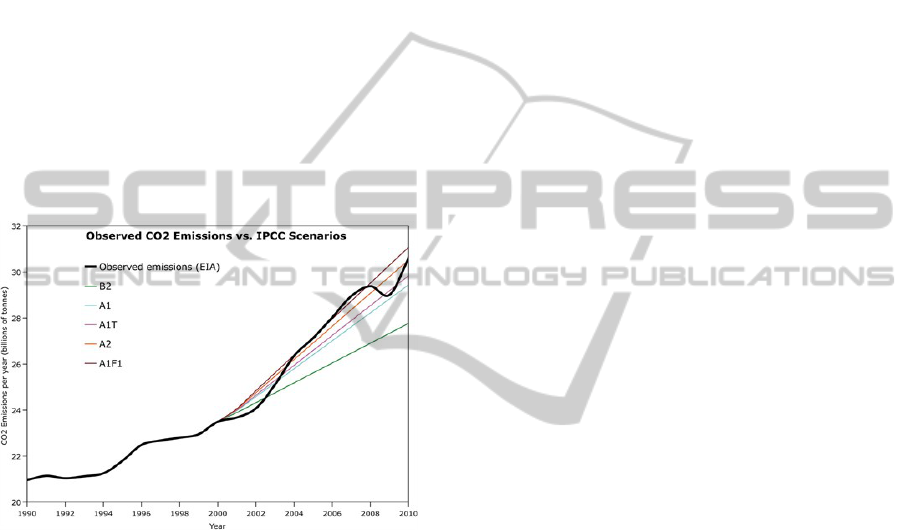
well below 400 ppmv by year 2100. The observed
emission pictured in figure 6 where the IPCC
scenarios are also shown are contained within A1F1
and the A1B therefore we could say that they point
to a temperature increase that will surpass the two
degrees. In fact to keep temperatures under 2
degrees we have already stated we should remain
under 400 ppmv and we are very very close (fuzzy
concept) to this concentration.
Figure 6: Observed CO2 emissions against IPCC AR4
scenarios (taken form http://www.treehugger.com/clean-
technology/iea-co2-emissions-update-2010-bad-news-
very-bad-news.html).
ACKNOWLEDGEMENTS
This work was supported by the Programa de
Investigación en Cambio Climático (PINCC,
www.pincc.unam.mx) of the Universidad Nacional
Autónoma de México.
REFERENCES
Dubois, D. and Prade, H. M., Fuzzy Sets and Systems:
Theory and Applications, Academic Press, 1980.
Gay, C., Estrada, F. 2009. Objective probabilities about
future climate are a matter of opinion. Climatic
Change, [http://dx.doi.org/10.1007/s10584-009-9681-
4].
IPCC-WGI, 2007: Climate Change 2007: The Physical
Science Basis. Contribution of Working Group I to the
Fourth Assessment Report of the Intergovernmental
Panel on Climate Change [Solomon, S., D. Qin, M.
Manning, Z. Chen, M. Marquis, K. B. Averyt, M.
Tignor and H. L. Miller (eds.)] Cambridge University
Press, Cambridge, United Kingdom and New York,
NY, USA, 996 pp.
IPCC-WGI, 2001: Climate Change 2001: The Scientific
Basis, Contribution of Working Group I to the Third
Assessment Report of the Intergovernmental Panel on
Climate Change, [Houghton, J.T.; Ding, Y.; Griggs,
D.J.; Noguer, M.; van der Linden, P.J.; Dai, X.;
Maskell, K.; and Johnson, C.A., ed.] Cambridge
University Press, ISBN 0-521-80767-0, (pb: 0-521-
01495-6).
Jaynes, E. T. 1957. Information Theory and Statistical
Mechanics: Phys. Rev., 106, 620-630.
Klir, G. and Elias, D. 2002. Architecture of Systems
Problem Solving, 2nd ed., NY: Plenum Press.
Nakicenovic, N., J. Alcamo, G. Davis, B. de Vries, J.
Fenhann, S. Gaffin, K. Gregory, A. Grübler, T. Y.
Jung, T. Kram, E. L. La Rovere, L. Michaelis, S.
Mori, T. Morita, W. Pepper, H. Pitcher, L. Price, K.
Riahi, A. Roehrl, H.-H. Rogner, A. Sankovski, M.
Schlesinger, P. Shukla, S. Smith, R. Swart, S. van
Rooijen, N. Victor, Z. Dadi, 2000. Special Report on
Emissions Scenarios: A Special Report of Working
Group III of the Intergovernmental Panel on Climate
Change. Cambridge University Press, Cambridge, 599
pp.
Ross, T. J. 2004. Fuzzy Logic with Engineering
Applications (2nd ed.) John Wiley & Sons.
Schneider, S. H., 2003. Congressional Testimony: U.S.
Senate Committee on Commerce, Science and
Transportation, Hearing on “The Case for Climate
Change Action” October 1, 2003.
Schmidt, G. A. 2007. The physics of climate modeling,
Phys. Today, 60, no. 1, 72-73.
Zadeh, L. A. 1965. Fuzzy Sets: Information and Control.
Vol. 8(3) p. 338-353.
APPENDIX
A.1 Fuzzy Logic Basic Concepts
As Klir stated in his book (Klir and Elias, 2002), the
view of the concept of uncertainty has been changed
in science over the years. The traditional view looks
to uncertainty as undesirable in science and should
be avoided by all possible means. The modern view
is tolerant of uncertainty and considers that science
should deal with it because it is part of the real
world. This is especially relevant when the goal is to
construct models. In this case, allowing more
uncertainty tends to reduce complexity and increase
SIMULTECH2012-2ndInternationalConferenceonSimulationandModelingMethodologies,Technologiesand
Applications
524
credibility of the resulting model. The recognition
by the researchers of the important role of
uncertainty mainly occurs with the first publication
of the fuzzy set theory, where the concept of objects
that have not precise boundaries (fuzzy sets) is
introduced (Zadeh, 1965).
Fuzzy logic, based on fuzzy sets, is a superset of
conventional two-valued logic that has been
extended to handle the concept of partial truth, i.e.
truth values between completely true and completely
false.
In classical set theory, when A is a set and x is an
object, the proposition “x is a member of A” is
necessarily true or false, as stated on equation 1,
⎩
⎨
⎧
∉
∈
=
Axfor
Axfor
xA
0
1
)(
(1)
whereas, in fuzzy set theory, the same proposition is
not necessarily either true or false, it may be true
only to some degree. In this case, the restriction of
classical set theory is relaxed allowing different
degrees of membership for the above proposition,
represented by real numbers in the closed interval
[0,1], i.e.
[]
1,0: →XA
. Figure A.1 presents this
concept graphically.
Figure A.1: Gaussian membership functions of a
quantitative variable representing ambient temperature.
Figure A.1 illustrates the membership functions
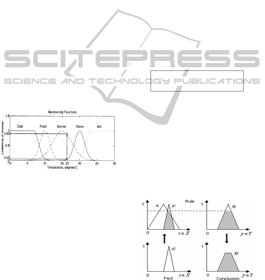
of the classes: cold, fresh, normal, warm, and hot, of
the ambient temperature variable. A temperature of
23°C is a member of the class normal with a grade
of 0.89 and a member of the class warm with a grade
of 0.05. The definition of the membership functions
may change with regard to who define them. For
example, the class normal for ambient temperature
variable in Mexico City can be defined as it is
shown in figure A.1. The same class in Anchorage,
however, will be defined more likely in the range
from -8°C to -2°C. It is important to understand that
the membership functions are not probability
functions but subjective measures. The opportunity
that brings fuzzy logic to represent sets as degrees of
membership has a broad utility. On the one hand, it
provides a meaningful and powerful representation
of measurement uncertainties, and, on the other
hand, it is able to represent efficiently the vague
concepts of natural language. Going back to the
example of figure A.1, it is more common and useful
for people to know that tomorrow will be hot than to
know the exact temperature grade.
At this point, the question is, once we have the
variables of the system that we want to study
described in terms of fuzzy sets, what can we do
with them? The membership functions are the basis
of the fuzzy inference concept. The compositional
rule of inference is the tool used in fuzzy logic to
perform approximate reasoning. Approximate
reasoning is a process by which an imprecise
conclusion is deduced from a collection of imprecise
premises using fuzzy sets theory as the main tool.
The compositional rule of inference translates the
modus ponens of the classical logic to fuzzy logic.
The generalized modus ponens is expressed by:
Rule: If X is A then Y is B
Fact: X is A'
Conclusion: Y is B'
where, X and Y are variables that take values from
the sets X and Y, respectively, and A, A' and B, B'
are fuzzy sets on X and Y, respectively. Notice that
the Rule expresses a fuzzy relation, R, on X x Y.
Then, if the fuzzy relation, R, and the fuzzy set
A' are given, it is possible to obtain B' by the
compositional rule of inference, given in equation 2,
[
]
),(),('minsup)(' yxRxAyB
Xx∈
=
(2)
where sup stands for supremum (least upper bound)
and min stands for minimum. When sets X and Y
are finite, sup is replaced by the maximum operator,
max. Figure A.2 illustrates in a simplified way the
compositional rule of inference graphically.
Figure A.2: Simplified graphical representation of the
compositional rule of inference.
SimpleFuzzyLogicModelstoEstimatetheGlobalTemperatureChangeDuetoGHGEmissions
525

The compositional rule of inference is also useful
in the general case where a set of rules, instead of
only one, define the fuzzy relation, R.
A.2 Extension Principle
Zadeh says that rather than regarding fuzzy theory as
a single theory, we should regard the conversion
process from binary to membership functions as a
methodology to generalize any specific theory from
a crisp (discrete) to a continuous (fuzzy) form. The
extension principle enables us to extend the domain
of a function on fuzzy sets, i.e., it allows us to
determine the fuzziness in the output given that the
input variables are already fuzzy. Therefore, it is a
particular case of the compositional rule of
inference. Figure A.3 gives a first idea of the
extension principle showing an example of two input
variables with 3 fuzzy sets each.
Figure A.3: Extension principle example for two input
fuzzy variables A and B with 3 fuzzy sets each.
The extension principle is applied to transform
each fuzzy pair (A
i
, B
j
), in a fuzzy set of the C
output variable. Notice that in the example of figure
A.3 we have 9 pairs of fuzzy input sets and,
therefore, 9 fuzzy sets are obtained representing the
conclusion as shown in the right hand side of figure
A.3. The extension principle when two input
variables are available is presented in equation 3. C
k
is the k
th
output fuzzy set extended from the two
input fuzzy sets A
i
and B
j
. In the example at hand, as
illustrated in figure A.3, the extension principle is
applied 9 times, to obtain each of the output fuzzy
sets associated to each fuzzy input pair.
(, )
max min ,
kij
kij
CfAB
CAB
=
⎡⎤
=
⎣⎦
(3)
For instance, the output fuzzy set C
9
, is obtained
when using the extension principle of equation 3
with the input fuzzy sets A
1
and B
3
(Klir and Elias,
2002); (Dubois and Prade, 1980); (Ross, 2004).
SIMULTECH2012-2ndInternationalConferenceonSimulationandModelingMethodologies,Technologiesand
Applications
526
