
Prediction of PM
2.5
Concentrations using Fuzzy Inductive Reasoning
in Mexico City
Àngela Nebot and Francisco Mugica
Soft Computing Research Group, Technical University of Catalonia, Jordi Girona Salgado 1-3, Barcelona, Spain
Keywords: Air Pollution Prediction, PM
2.5
Pollution, Fuzzy Inductive Reasoning (FIR), Time Series Analysis.
Abstract: The research presented in this paper is focused on the study and development of fuzzy inductive reasoning
models that allow the forecasting of daily particulate matter with diameter of 2.5 micrometres or less
(PM2.5). FIR offers a model-based approach to modelling and predicting either univariate or multivariate
time series. In this research, predictions of PM
2.5
concentration at hour 12 of the next day, in the downtown
of Mexico City Metropolitan Area, are performed. The data were registered every hour and include missing
values. In this work the hourly modelling perspective is analyzed. The results are compared with the ones
obtained using persistence models showing that the FIR models are able to predict PM
2.5
concentrations
more accurately than persistence models.
1 INTRODUCTION
The high levels of particulate matter in the air are of
high concern since they may produce severe public
health effects and are the main cause of the
attenuation of visible light. There are very high
levels of particles in North Africa, much of the
Middle East, Asia, Latin America as well as in the
large urban areas. Comparing it with population
density maps, the WHO concluded that more than
80% of the world population is exposed to high
levels of fine particles (PM
2.5
) (WHO, 2006).
Likewise, identifies PM
2.5
as an important indicator
of risk to health and might also be a better indicator
than PM
10
for anthropogenic suspended particles in
many areas (van Donkelaar et al., 2010). According
to the WHO Guidelines, concentrations at this level
and higher are associated with an approximately
15% increased risk of mortality, relative to the Air
Quality Guideline (AQG) of 10 μg m
-3
(WHO,
2006).
Regarding the PM
2.5
, it has not yet been
identified a threshold below which damage to health
does not occur, this has motivated that the limits for
the protection of public health are getting lower
every year.
The geographical characteristics of the
Mexico city metropolitan area, i.e. its height,
average temperature and terrain, added to the
pressure exerted by the growth and intensification of
urban activities cause high air pollution episodes that
constitute a permanent challenge to the health of its
inhabitants. Although the measures taken over the
past 15 years to reduce the impact of air pollution
have managed to significantly decrease pollutants
such as SO2, CO or the Pb, the concentrations of
ozone and fine particles exceed quite often air
quality standards.
The monitoring of PM
2.5
from 2004 to date
shows that around 20 million people in Mexico city
are exposed to annual average concentrations of this
contaminant in between 19 and 25 μg m
-3
, exceeding
by more than double the WHO standard of 10 μg m
-3
and substantially exceeding the Mexican norm of 15
μg m
-3
.
The increase of the concentration of particles in
Mexico city is strongly associated with the
meteorology of the Valley. During the days of
intense wind, resuspension of dust from the ground
produces significant increases in the concentrations
of total suspended particles (PST) and particles
lower than 10 μm (PM
10
). The presence of surface
thermal inversions can contribute to the increase in
the concentration of particles smaller than 10 μm
and fine particles, due to the lack of dispersion and
the accumulation in the atmosphere of the particles
emitted by vehicles and industry. Higher
concentrations usually occur when the layer trapped
under the inversion is not very high and the duration
of the thermal inversion is maintained throughout
the morning.
527
Nebot À. and Mugica F..
Prediction of PM2.5 Concentrations using Fuzzy Inductive Reasoning in Mexico City.
DOI: 10.5220/0004165705270533
In Proceedings of the 2nd International Conference on Simulation and Modeling Methodologies, Technologies and Applications (MSCCEC-2012), pages
527-533
ISBN: 978-989-8565-20-4
Copyright
c
2012 SCITEPRESS (Science and Technology Publications, Lda.)

The national weather service reported a total of
107 days with surface thermal inversions during
2010, the highest in the past 13 years. The largest
part was recorded during the winter months, when
the long and cold nights favor its formation. In the
dry season months it has been reported a 40% of
days with thermal inversion. The months of April
and December had the largest number of events with
16 and 17 days, respectively. The influence of high
pressure systems during the months of March to
May was responsible for the formation of surface
thermal inversions (NWM, 2012).
In this research we propose predictions models
of hourly concentrations of PM
2.5
, based on data
obtained at downtown Mexico city. We show results
obtained with two different methods, all of which
use past values of PM
2.5
as input. The simplest
method is persistence, which assigns hourly values
on the next day equal to the values at the present
day. Then we used the fuzzy inductive reasoning
approach that is a non-linear methodology based on
fuzzy logic and pattern recognition. We used
registered data of 4 year periods, each lasting six
months starting on December 1
st
. As explained
before, the months from December to May are the
ones that have higher levels of PM
2.5
concentrations
in Mexico city metropolitan area.
In section 2 some basic concepts of the fuzzy
inductive reasoning approach are introduced. In
section 3 the methodology used is described, i.e. the
data, the fuzzy models development and the models
evaluation. Section 4 describes the results obtained.
Finally the conclusions of this research are given.
2 FUZZY INDUCTIVE
REASONING (FIR)
The conceptualization of the FIR methodology
arises of the General System Problem Solving
(GSPS) approach proposed by Klir (Klir and Elias,
2002). This methodology of modeling and
simulation is able to obtain good qualitative
relations between the variables that compose the
system and to infer future behavior of that system.
It has the ability to describe systems that cannot
easily be described by classical mathematics or
statistics, i.e. systems for which the underlying
physical laws are not well understood.
The Fuzzy Inductive Reasoning (FIR)
methodology, offers a model-based approach to
predicting either univariate or multi-variate time
series (Nebot et al., 2003); (Carvajal and Nebot,
1998). A FIR model is a qualitative, non-
parametric, shallow model based on fuzzy logic.
Fuzzy logic-based methods have not been applied
extensively in environmental science, however,
some interesting research can be found in the area
of modeling of pollutants (Mintz et al., 2005);
(Ghiaus, 2005); (Morabito and Versaci, 2003);
(Heo and Kim, 2004); (Yildirim and Bayramoglu,
2006); (Peton et al., 2000); (Onkal-Engin et al.,
2004), where different hybrid methods that make
use of fuzzy logic are presented for this task.
Visual-FIR is a tool based on the Fuzzy
Inductive Reasoning (FIR) methodology (runs under
Matlab environment), that offers a new perspective
to the modeling and simulation of complex systems.
Visual-FIR designs process blocks that allow the
treatment of the model identification and prediction
phases of FIR methodology in a compact, efficient
and user friendly manner (Escobet et al., 2008).
The FIR model consists of its structure (relevant
variables) and a set of input/output relations (history
behavior) that are defined as if-then rules. Feature
selection in FIR is based on the maximization of the
models' forecasting power quantified by a Shannon
entropy-based quality measure. The Shannon
entropy measure is used to determine the uncertainty
associated with forecasting a particular output state
given any legal input state. The overall entropy of
the FIR model structure studied, H
s,
is computed as
described in equation 1.
()
s
i
i
HpiH
∀
=
−⋅
∑
,
(1)
where p(i ) is the probability of that input state to
occur and H
i
is the Shannon entropy relative to the
i
th
input state. A normalized overall entropy H
n
is
defined in equation 2.
max
1
s
n
H
H
H
=−
(2)
H
n
is obviously a real-valued number in the range
between 0.0 and 1.0, where higher values indicate an
improved forecasting power. The model structure
with highest H
n
value generates forecasts with the
smallest amount of uncertainty.
Once the most relevant variables are identified,
they are used to derive the set of input/output
relations from the training data set, defined as a set
of if-then rules. This set of rules contains the
behaviour of the system. Using the five-nearest-
neighbors (5NN) fuzzy inferencing algorithm the
five rules with the smallest distance measure are
selected and a distance-weighted average of their
SIMULTECH2012-2ndInternationalConferenceonSimulationandModelingMethodologies,Technologiesand
Applications
528
fuzzy membership functions is computed and used
to forecast the fuzzy membership function of the
current state, as described in equation 3.
5
1
new j j
out rel out
j
M
emb w Memb
=
=⋅
∑
(3)
The weights
j
rel
w
are based on the distances and
are numbers between 0.0 and 1.0. Their sum is
always equal to 1.0. It is therefore possible to
interpret the relative weights as percentages.
For a more detailed explanation of the fuzzy
inductive reasoning methodology refer to (Escobet
et al., 2008).
3 METHODOLOGY
3.1 Data
The data used for this study stems from the
Atmospheric Monitoring System of Mexico City
(SIMAT in Spanish) that measures contaminants
and atmospheric variables from 36 stations
distributed through the 5 regions of the Mexico
City metropolitan area (SIMAT, 2012). The
registered variables are the air pollutants, including
PM
2.5
, as well as other 10 contaminants, and
meteorological variables, 24 hours a day, every day
of the year. The web page of SIMAT (SIMAT,
2012) offers a data base with meteorological and
contaminant registers since 1986 up to date,
although PM
2.5
has been registered for the first time
in 2004.
A mechanically oscillated mass balance type
instrument, TEOM 1400a, is used for the
registration of the PM
2.5
. This instrument is very
sensitive to changes in concentrations of mass and
can provide accurate measurements for samples
with less than an hour in length.
This study is centered on the univariate modeling
and forecasting of particulate matter with diameter
of 2.5 micrometres or less (PM
2.5
) in the Merced
station, located in the commercial and administrative
district at the downtown of Mexico City
Metropolitan Area (MCMA).
The PM
2.5
variable
is an hourly instantaneous
observation, not the maximum or the mean of
minute registered data. We have chosen to work
with the scalar time series on PM
2.5
concentrations
keeping in mind the idea that if we use a large
enough window of data as input, the effect of other
pollutants or meteorological data should be implicit
in its structure (Pérez et al., 2000).
The typical pattern of PM
2.5
from some city
areas, such is for example downtown, suggests that
concentrations of this contaminant increase regularly
between 8:00 and 16:00 hours, with maximum
concentrations around 13:00 hours
(Muñoz et al.,
2000).
Therefore, we have decided to use in this study
data from the half of the year that Mexico city
suffers higher PM
2.5
concentrations, i.e. from
December to May. We have used 4 data sets
containing 6 month of hourly registers each one,
i.e. from the 1
st
of December until de 31
st
of May,
for years 2007-2008, 2008-2009, 2009-2010 and
2010-2011.
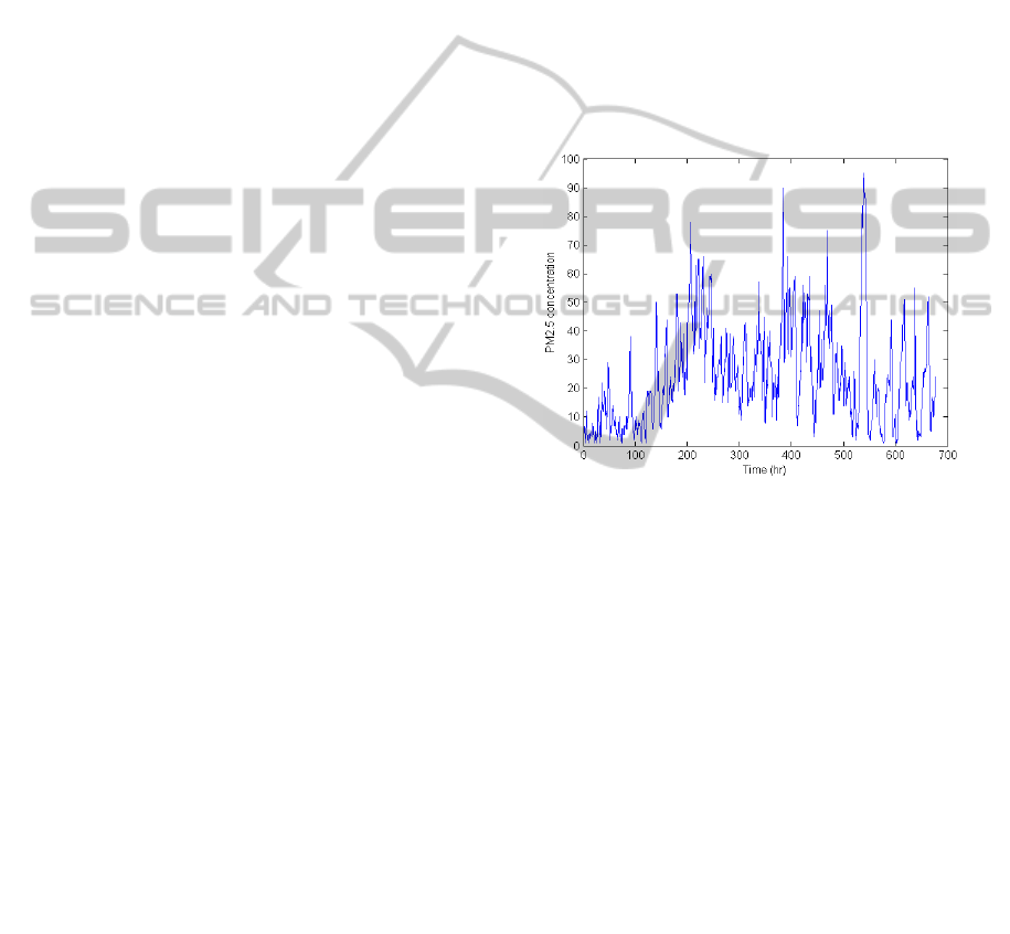
Figure 1: Hourly concentrations of PM
2.5
data for
December 2009. Units are µg m
-3
. From the 720 data
points, 42 are missing values that are not plotted.
For the first data set, i.e. 1
st
December 2007 to
31
st
May 2008, the average concentration is 31.2 µg
m
-3
, the maximum is 147 µg m
-3
and the standard
deviation is 15.6 µg m
-3
. For the second data set, i.e.
1
st
December 2008 to 31
st
May 2009, the average
concentration is 26.6 µg m
-3
, the maximum is 102
µg m
-3
and the standard deviation is 14.3 µg m
-3
.
For the third data set, i.e. 1
st
December 2009 to
31
st
May 2010, the average concentration is 20.8 µg
m
-3
, the maximum is 101 µg m
-3
and the standard
deviation is 13.4 µg m
-3
. For the last data set, i.e. 1
st
December 2010 to 31
st
May 2011, the average
concentration is 32.5 µg m
-3
, the maximum is 175
µg m
-3
and the standard deviation is 16.5 µg m
-3
.
Fig. 1 shows the hourly concentrations of PM
2.5
during December, 2009.
The data available contains missing values that
correspond to data that was not registered due to
instrument problems. From the total number of
17496 hourly data registered, 1316 are missing
values.
PredictionofPM2.5ConcentrationsusingFuzzyInductiveReasoninginMexicoCity
529

3.2 Fuzzy Models Development
As mentioned before, our goal is to obtain FIR
models capable of forecasting the PM
2.5
concentrations some time in advance, in such a way
that efficient actions could be taken in order to
protect the citizens of high concentrations episodes.
We first performed a study of the
autocorrelation, both causal and temporal, of the
PM
2.5
time series. To this end, we used the model
structure identification process of the fuzzy
inductive reasoning methodology that performs a
feature selection based on the entropy reduction
measure, described in section 2.
We have found that it is possible to relate the
concentration of PM
2.5
at a given time of the day to
the sequence of 24 points corresponding to the
hourly concentrations on the previous day.
Moreover, the structure of the fuzzy inductive
reasoning model has determined that there is a direct
causal relation between the level of pollution at
present time and its values at hours 6, 12, 18 and 24.
That is, there is a positive correlation at hours 12 and
24 and a negative correlation at hours 6 and 18.
With this information available we think that an
interesting and useful approximation to modeling
and forecasting PM
2.5
concentrations is to obtain a
model for each hour of the day, based on the values
of the 6, 12, 18 and 24 hours of the previous day, i.e.
hourly models.
In order to study this approach, in this research
we have developed FIR models for the prediction of
hour 12 of the next day (FIR-12). The input
variables of the system are PM
2.5
concentration at
hours 6, 12, 18 and 24. Therefore, we have 4 input
variables. The output variable is PM
2.5
concentration
at hour 12 of the next day. Therefore, for this FIR
prediction model, pollutant concentrations are given
12h in advance.
We plan to obtain FIR models, in the near future,
for each hour of the day, i.e. FIR-1 to FIR-24,
predictions will be made from 1 to 24 h in advance,
respectively.
In order to obtain the FIR-12 model it is
necessary to arrange the data in such a way that we
have a data stream for each day instead of 24 data
streams (one for each hour of that day).
The 4 data sets available have been arranged
accordingly, obtaining now a total number of 725
daily data, out of which 220 are missing values.
In this work a 10-fold cross validation is used to
assess how the results of the obtained models will
generalize to an independent data set. The objective
is to estimate how accurately the predictive models
developed in this study will perform in practice. As
described before, 505 data points are available, i.e.
725 minus 220 missing. Therefore, 10 test sets with
50 data points and 10 training sets with 450 data
points are used.
The first step in order to obtain the FIR-12 model
is to convert quantitative values in fuzzy data, to this
end, it is necessary to specify two discretization
parameters, i.e. the number of classes per system
variable (granularity) and the membership functions
(landmarks) that define its semantics. In this study
the granularity and the clustering method used to
obtain the landmarks are summarized in table 1. Half
of the folds are discretized into two classes using the
fuzzy c-means clustering method. It is not possible
to use more classes in this case because the number
of training data (450 points) is not larger enough.
Other clustering methods such are median linkage,
k-means and equal frequency partition are also used
in this study. However, no one of these methods take
into account the uncertainty associated to the data in
order to obtain the landmarks parameter.
Table 1: Interval values (landmarks) associated to each
class for input and output variables.
Number
classes
Clustering method
FOLD 1, 5, 7, 8, 9 2 Fuzzy C-means
FOLD 2, 6 3 Equal Frequency Partition
FOLD 3, 10 2 Median Linkage
FOLD 4 2 K-Means
The FIR model structure obtained in this case
may be described using the scheme shown in
equation 4.
),,,(
2418126
xxxxfy
qt
=
(4)
where y
t
is the predicted value at time t on the
following day; x
i
represent the pollution data on a
given day at the i
th
hour; and f
q
is the qualitative
relation of the FIR model. We focus this research in
FIR models for t=12.
3.3 Model Evaluation
Two error measures were used to evaluate the
performance of each of the FIR-12 models. These
are: the root mean square error and the mean
absolute error. The root mean square error (RMSE)
is described in equation 5.
()
2
1
ˆ
() ()
N
ii
i
yt yt
RMSE
N
=
−
=
∑
(5)
SIMULTECH2012-2ndInternationalConferenceonSimulationandModelingMethodologies,Technologiesand
Applications
530

where ŷ (t) is the predicted output, y(t) the system
output and N the number of samples.
The mean absolute error (MAE) is defined in
equation 6.
1
1
ˆ
() ()
N
ii
i
M
AE y t y t
N
=
=−
∑
(6)
4 RESULTS AND DISCUSSION
The results obtained by the FIR models are
compared with the ones obtained when using the
persistence method. This consist of a very simple
prediction, i.e. tomorrow at time t PM
2.5
mass
concentration will be the same as today at time t. In
this case equation 4 takes the form of equation 7.
tt
xy =
(7)
Therefore, there are no parameters to adjust. The
prediction results obtained by FIR and persistence
models of the
PM
2.5
contaminant at hour 12 of the
next day, for each fold, are summarized in table 2.
Table 2: Prediction errors of each fold separately and its
average for the PM
2.5
concentration series. Predictions are
at hour 12 of the next day using FIR and persistence
models. The inputs of the FIR models are PM
2.5
at hours 6,
12, 18 and 24 today.
MAE
FIR
MAE
PERS.
RMSE
FIR
RMSE
PERS.
FOLD 1
(1-50)
15.9 19.9 20.9 24.0
FOLD 2
(51-100)
13.6 13.7 17.6 18.3
FOLD 3
(101-150)
10.8 13.5 14.1 17.1
FOLD 4
(151-200)
13.3 14.7 16.8 18.6
FOLD 5
(201-250)
9.5 9.8 13.5 14.1
FOLD 6
(251-300)
17.0 19.7 21.9 26.8
FOLD 7
(301-350)
12.0 10.1 14.7 13.4
FOLD 8
(351-400)
19.0 22.1 25.1 31.4
FOLD 9
(401-450)
11.9 13.4 15.4 18.1
FOLD 10
(451-505)
11.9 13.1 15.5 17.0
MEAN
FOLDS
13.5 16.5 17.5 19.9
From table 2 it can be seen that FIR models
perform much better than persistence, for all the
folds except for fold 7. Notice, that the range below
the number of the fold means the set of forecasted
data. The mean prediction errors are significantly
lower for the FIR models, i.e. 13.5 vs. 16.5 of MAE
and 17.5 vs. 19.9 of RMSE. However,
t
he accuracy
of the predictions produced with the FIR models is
probably poor in order for the results to have
practical application in environmental pollution
policies.
In order to try to enhance the previous results we
have considered including meteorological variables
in the study. Cobourn concludes that the
meteorological variables that have a nonlinear
relationship
with PM
2.5
statistically significant are
maximum temperature and wind speed. Moreover,
the strongest single relationship between PM
2.5
and
any one meteorological variable is the
relationship
with daily maximum temperature (Cobourn, 2010).
Therefore, the next step in our research was to
study the prediction capability of the models when
the maximum temperature of the day is also
considered as an input variable.
In this case, the number of missing values
increases and instead of 505 data available we only
have 481. Therefore, each fold of the 10-fold cross
validation has now 48 data points.
The FIR model structure obtained in this case
may be described using the scheme shown in
equation 8.
),,,,(
2418126
zxxxxfy
qt
=
(8)
where y
t
is the predicted value at time t on the
following day; x
i
represent the pollution data on a
given day at the i
th
hour; z is the maximum
temperature on a given day; f
q
is the qualitative
relation of the FIR model.
Table 3: Interval values (landmarks) associated to each
class for input and output variables.
Number
classes
Clustering method
FOLD 1, 4, 8, 9 2 Fuzzy C-means
FOLD 2, 6, 7 2 and 3 Equal Frequency Partition
FOLD 3 2 Median Linkage
FOLD 5 2 K-Means
The granularity and the clustering method used
to obtain the landmarks in this case are summarized
in table 3.
Table 4 shows the prediction results obtained by
FIR and persistence models of the PM
2.5
contaminant
at hour 12 of the next day, for each fold, when the
inputs of the model are: PM
2.5
at hours 6, 12, 18 and
24 and maximum temperature today.
As can be seen for the prediction errors of table 4
the inclusion of today’s temperature as input
PredictionofPM2.5ConcentrationsusingFuzzyInductiveReasoninginMexicoCity
531

variable of the model does not enhance substantially
the accuracy of FIR-12 models.
Table 4: Prediction errors of each fold separately and its
average for the PM
2.5
concentration series. Predictions are
at hour 12 of the next day using FIR and persistence
models. The inputs of the FIR models are PM
2.5
at hours 6,
12, 18 and 24 and maximum temperature today.
MAE
FIR
MAE
PERS.
RMSE
FIR
RMSE
PERS.
FOLD 1
(1-48)
17.1 20.4 21.4 24.4
FOLD 2
(49-96)
11.5 11.4 14.4 15
FOLD 3
(97-144)
11 13.8 13.8 17.7
FOLD 4
(145-192)
12.7 14.5 16.7 18.5
FOLD 5
(193-240)
10.6 9.5 14 14
FOLD 6
(241-288)
16.7 20.5 21.9 27.4
FOLD 7
(289-336)
10.4 10.3 12.7 13.6
FOLD 8
(337-384)
15.9 19.5 21.1 28.8
FOLD 9
(385-432)
11.6 12.7 15.7 17.3
FOLD 10
(433-481)
11.5 13.6 14.3 17.6
MEAN
FOLDS
12.9 14.6 16.6 18.4
PM
2.5
is a difficult contaminant to be predicted
due to the fact that there are significant variations of
the concentrations of this pollutant from one day to
the next day, and, from one hour to the next one,
even with similar weather conditions.
Previous works have been focused on the
modelling and prediction of mean (Kang et al.,
2010) or maximum (Cobourn, 2010) PM
2.5
concentrations. Also, there are studies that perform
binary predictions, i.e. if a dangerous level has been
reached (Dong et al., 2009). Contrarily, we have
focused on a short-term PM
2.5
forecast, although
uncertainties in hourly registers pose enormous
challenges for developing accurate models.
5 CONCLUSIONS
In this paper PM
2.5
models based on the fuzzy
inductive reasoning approach were developed for
downtown Mexico city metropolitan area, to predict
the concentration of this contaminant at hour 12 of
the next day.
The results obtained are better than the
predictions encountered by persistence models.
However, we think that the accuracy reached is still
poor for the results to have practical application in
environmental policies.
In order to enhance the predictions the maximum
temperature has been used as an additional input
variable. The prediction errors are quite similar to
the ones obtaind by the FIR models when only PM
2.5
is used.
As a future work we propose to:
• Include other meteorological variables into the
model.
• Include additional information such are day of
the week or hour of the day into the models.
• Develop models for all the hours of the day, in
such a way that predictions will be from 1 to 24
hours in advance.
• Use hybrid modelling techniques such as fuzzy
inductive reasoning with genetic algorithm, which
will help to find in an efficient way the number of
classes and landmarks parameters of FIR
discretization process.
REFERENCES
Carvajal, R., Nebot, A., 1998. Growth Model for White
Shrimp in Semi-intensive Farming using Inductive
Reasoning Methodology. Computers and Electronics
in Agriculture 19, 187-210.
Cobourn, W. G., 2010. An enhanced PM2.5 air quality
forecast model based on nonlinear regression and
back-trajectory concentrations. Atmospheric
Environment 44, 3015-3023.
Dong, M., Yang, D., Kuang. Y., He, D., Erdal, S., Kenski,
D., 2009. PM
2.5
concentration prediction using hidden
semi-Markov model-based times series data mining.
Expert Systems with Applications 36, 9046-9055.
Escobet, A., Nebot., A., Cellier, F. E., 2008. Visual-FIR:
A tool for model identification and prediction of
dynamical complex systems. Simulation Modelling
Practice and Theory 16, 76-92.
Ghiaus, C., 2005. Linear fuzzy-discriminant analysis
applied to forecast ozone concentration classes in sea-
breeze regime. Atmospheric Environment 39, 4691-
4702.
Heo, J. S., Kim, D. S., 2004. A new method of ozone
forecasting using fuzzy expert and neural network
system. Sicence of the Total Environment 325, 221-
237.
Kang, D., Mathur, R., Trivikrama Rao, S., 2010.
Assessment of bias-adjusted PM
2.5
air quality forecast
over the continental United States during 2007.
Geoscience Model Dev. 3, 309-320.
Klir, G., Elias, D., 2002. Architecture of Systems Problem
Solving, Plenum Press. New York, 2
nd
edition.
Mintz, R., Young, B.R., Svrcek, W.Y., 2005. Fuzzy logic
SIMULTECH2012-2ndInternationalConferenceonSimulationandModelingMethodologies,Technologiesand
Applications
532

modeling of surface ozone concentrations. Computers
& Chemical Engineering 29, 2049-2059.
Morabito, F. C., Versaci, M., 2003. Fuzzy neural
identification and forecasting techniques to process
experimental urban air pollution data. Neural
Networks 16, 493-506.
Muñoz, R., Carmona, M. R., Pedroza, J.L., Granados,
M.G., 2000. Data analysis of PM2.5 registered with
TEOM equipment in Azcapotzalco (AZC) and St.
Ursula (SUR) stations of the automatic air quality
monitoring network (RAMA). In: National Congress
of Medicine Engineering and Ambient Sciences, 21-
24. In Spanish.
NWM: National Weather Service of Mexico, 2012:
http://smn.cna.gob.mx/
Nebot, A., Mugica, F., Cellier, F., Vallverdú, M., 2003.
Modeling and Simulation of the Central Nervous
System Control with Generic Fuzzy Models.
Simulation 79(11), 648-669.
Onkal-Engin, G., Demir, I., Hiz, H., 2004. Assessment of
urban air quality in Istanbul using fuzzy synthetic
evaluation. Atmospheric Environment 38, 3809-3815.
Pérez, P., Trier, A., Reyes, A., 2000. Prediction of PM2.5
concentrations several hours in advance using neural
networks in Santiago, Chile. Atmospheric
Environment 34, 1189-1196.
Peton, N., Dray, G., Pearson, D., Mesbah, M., Vuillot, B.,
2000. Modelling and analysis of ozone episodes.
Environmental Modelling & Software 15, 647-652.
SIMAT, www.sma.df.gob.mx/simat/, 2012.
WHO World healt oranization (2006). Air quality
guidelines: the global update 2005
Yildirim, Y., Bayramoglu, M., 2006. Adaptive neuro-
fuzzy based modelling for prediction of air pollution
daily levels in city of Zonguldak. Chemosphere 63,
1575-1582.
PredictionofPM2.5ConcentrationsusingFuzzyInductiveReasoninginMexicoCity
533
