Evidence Accumulation Clustering using Pairwise Constraints
Jo
˜
ao M. M. Duarte
1,2
, Ana L. N. Fred
2
and F. Jorge F. Duarte
1
1
GECAD - Knowledge Engineering and Decision Support Group,
Institute of Engineering, Polytechnic of Porto (ISEP/IPP), Porto, Portugal
2
Instituto de Telecomunicac¸
˜
oes, Instituto Superior T
´
ecnico, Lisboa, Portugal
Keywords:
Constrained Data Clustering, Clustering Combination, Unsupervised Learning.
Abstract:
Recent work on constrained data clustering have shown that the incorporation of pairwise constraints, such as
must-link and cannot-link constraints, increases the accuracy of single run data clustering methods. It was also
shown that the quality of a consensus partition, resulting from the combination of multiple data partitions, is
usually superior than the quality of the partitions produced by single run clustering algorithms. In this paper we
test the effectiveness of adding pairwise constraints to the Evidence Accumulation Clustering framework. For
this purpose, a new soft-constrained hierarchical clustering algorithm is proposed and is used for the extraction
of the consensus partition from the co-association matrix. It is also studied whether there are advantages in
selecting the must-link and cannot-link constraints on certain subsets of the data instead of selecting these
constraints at random on the entire data set. Experimental results on 7 synthetic and 7 real data sets have
shown the use of soft constraints improves the performance of the Evidence Accumulation Clustering.
1 INTRODUCTION
Data clustering is an unsupervised learning discipline
which aims to discover structure in data. A clustering
algorithm groups a set of unlabeled data patterns into
meaningful clusters using some notion of similarity
between data, so that similar patterns are placed in
the same cluster and dissimilar patterns are assigned
to different clusters.
Inspired by the success of the supervised classi-
fier ensemble methods, many unsupervised clustering
ensemble methods were proposed in the last decade.
The idea is to combine multiple data partitions to im-
prove the quality and robustness of data clustering
(Fred, 2001), to reuse existing data partitions (Strehl
and Ghosh, 2003), and to partition data in a dis-
tributed way. The clustering ensemble methods can
be categorized according to the way the clustering en-
semble is build: one or several clustering algorithms
can be applied, using different parameters and initial-
izations (Fred and Jain, 2005), different subsets of
data patterns (Topchy et al., 2004) or attributes, and
projections of the original data representation into an-
other spaces (Fern and Brodley, 2003); and regard-
ing how the consensus partition is obtained: by ma-
jority voting (Dudoit and Fridlyand, 2003), by using
the associations between pairs of patterns (Fred and
Jain, 2005), finding a median partition (Topchy et al.,
2003), and mapping the clustering ensemble problem
into graph (Fern and Brodley, 2004; Domeniconi and
Al-Razgan, 2009) or hypergraph (Strehl and Ghosh,
2003) formulations.
Recently, some researchers focused on including
some a priori knowledge about the data into clus-
tering (Basu et al., 2008). Constrained data cluster-
ing maps this knowledge as constraints to be used
by a constrained clustering algorithm. These con-
straints manifest the preferences, limitations or con-
ditions that a user may want to impose in the clus-
tering solution, so that the clustering solution may
be more useful for each particular case. Some con-
strained data clustering algorithms have already been
proposed regarding distinct perspectives: inviolable
constraints (Wagstaff, 2002), distance editing (Klein
et al., 2002), using partial label data (Basu, 2005),
penalizing the violation of constraints (Davidson and
Ravi, 2005), modifying the generation model (Basu,
2005), and encoding constraints into spectral cluster-
ing (Wang and Davidson, 2010).
In this paper, we explore the use of pairwise
constraints in the Evidence Accumulation Clustering
framework. A constrained clustering algorithm is pro-
posed and used to produce consensus partitions. The
effect of acquiring constraints involving objects easy
293
M. M. Duarte J., L. N. Fred A. and F. Duarte F..
Evidence Accumulation Clustering using Pairwise Constraints.
DOI: 10.5220/0004171902930299
In Proceedings of the International Conference on Knowledge Discovery and Information Retrieval (KDIR-2012), pages 293-299
ISBN: 978-989-8565-29-7
Copyright
c
 2012 SCITEPRESS (Science and Technology Publications, Lda.)

and/or hard to cluster is also investigated.
The remaining of the paper is organized as fol-
lows. In section 2, the clustering combination
problem and the Evidence Accumulation Clustering
method are described in subsection 2.1, the incorpo-
ration of constraints in Evidence Accumulation Clus-
tering is explained in subsection 2.2, and an soft-
constrained hierarchical clustering algorithm is pro-
posed in subsection 2.3. The process of acquiring
pairwise constraints is presented in section 3. In sec-
tion 4 the experimental setup of our work is described
and the experimental results are presented. Section 6
concludes this paper.
2 EVIDENCE ACCUMULATION
CLUSTERING USING
PAIRWISE CONSTRAINTS
2.1 Combination of Multiple Data
Partitions
Let X = {x
1
, ··· , x
n
}be a data set with n data patterns.
A clustering algorithm divides the data set X into K
clusters resulting in a data partition P = {C
1
, ··· ,C
K
}.
By changing the algorithm parameters and/or initial-
izations different partitions of X can be obtained. A
clustering ensemble P = {P
1
, ··· , P
N
} is defined as
a set of N data partitions of X . Consensus clustering
methods, also known as clustering combination meth-
ods, use the information contained in P to produce a
consensus partition P
∗
.
One of the most known clustering combination
methods is the Evidence Accumulation Clustering
method (EAC) (Fred and Jain, 2005). EAC treats each
data partition P
l
∈ P as an independent evidence of
data organization. The key idea is that if two data pat-
terns are frequently co-assigned to the same clusters
in P than they probably belong to the same “natural”
cluster.
EAC uses a n ×n co-association matrix C to keep
the frequency that each pair of patterns is grouped into
the same cluster. The co-association matrix is com-
puted as
C
i j
=
∑
N
l=1
vote
l
i j
N
, (1)
where vote
l
i j
= 1 if x
i
, and x
j
co-occur in a cluster
of data partition P
l
and vote
l
i j
= 0 otherwise. After
the co-association matrix have been computed, it is
used as input to a clustering algorithm to produce the
consensus partition P
∗
.
2.2 Clustering with Constraints
Different types of constraints can be used to influ-
ence the data clustering solution. At a more general
level, constraints may be applied to the entire data set.
An example of this type of constraints is data clus-
tering with obstacles (Tung et al., 2000). The con-
straints may be used at an intermediate level, where
they may be applied to mold the characteristics of the
clusters, such as the minimum and maximum capacity
(Ge et al., 2007), or to data features (Wagstaff, 2002).
At a more specific level, the constraints may be em-
ployed at the level of the individual data patterns, us-
ing labels on some data (Basu, 2005) or defining rela-
tions between pairs of patterns (Wagstaff, 2002), such
as must-link and cannot-link constraints. We will fo-
cus on these relations between pairs of patterns due
to their versatility: many constraints on more gen-
eral levels can easily be converted to must-link and
cannot-link constraints.
The relations between pair of clusters are repre-
sented by two sets: the set of must link constraints
(R
=
) and the set of cannot-link (R
6=
) constraints. On
one hand, to indicate that two data patterns, x
i
and
x
j
, should belong to the same cluster a must-link con-
straint between x
i
and x
j
should be added to R
=
. On
the other hand, if x
i
should not be placed in the clus-
ter of x
j
a cannot-link constraint should be added to
R
6=
. These instance level constraints can be regarded
as hard or soft constraints, whether the constraint sat-
isfaction is mandatory or not.
To incorporate pairwise constraints in the Evi-
dence Accumulation Clustering framework, we sim-
ple apply a pairwise-constrained clustering algorithm
to the co-association matrix, as suggested in (Duarte
et al., 2009). For this purpose, a modification to the
average-link (Sokal and Michener, 1958) algorithm
is proposed in subsection 2.3. Figure 1 summarizes
the Constrained Evidence Accumulation Clustering
model. In the first step, the Clustering Generation
Step, one or several clustering algorithms using differ-
ent parameters and initializations are used to produce
N partitions of the given data set. Then, in the Con-
sensus Step, the co-association matrix is built as de-
scribed in subsection 2.1, and a constrained clustering
algorithm uses the information contained in the co-
association matrix and the set of pairwise constraints
to produce the consensus partition.
2.3 Soft-constrained Average-link
Clustering Algorithm
An agglomerative hierarchical clustering algorithm
starts with n clusters, where each cluster is composed
KDIR2012-InternationalConferenceonKnowledgeDiscoveryandInformationRetrieval
294

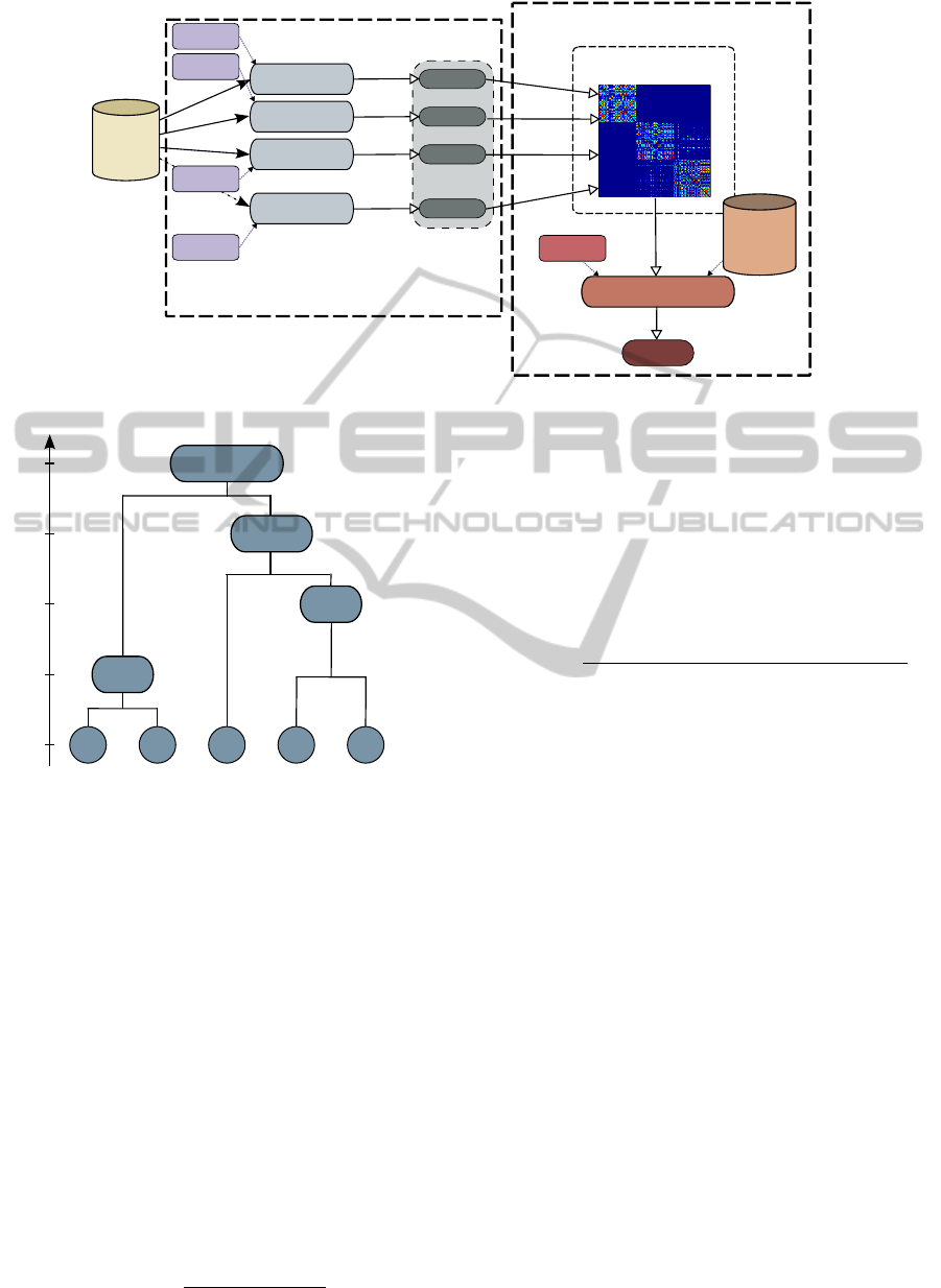
Data set
Clustering
Algorithm 1
Clustering
Algorithm 2
Clustering
Algorithm 3
Clustering
Algorithm N
...
Parameters
Set 1
Parameters
Set 2
Parameters
Set N
Parameters
Set 3
Partition 1
Partition 2
Partition 3
Partition N
...
Clustering
Ensemble
Co-association
Matrix
Constrained
Clustering Algorithm
Parameters
Set
Consensus
Partition
Clustering Generation Step
Consensus Step
...
Set of
Constraints
Figure 1: Constrained Evidence Accumulation Clustering Model.
{x
1
} {x
2
} {x
3
} {x
4
} {x
5
}
{x
1
,x
2
}
{x
4
,x
5
}
{x
3
,x
4
,x
5
}
{x
1
,x
2
,x
3
,x
4
,x
5
}
Step 0 Step 1 Step 2 Step 3 Step 4
Figure 2: Example of a dendrogram produced by an ag-
glomerative clustering algorithm.
of a single data pattern, i.e. ∀x
i
∈ X ,C
i
= {x
i
}. Then,
iteratively, the two closest clusters according to some
distance measure between clusters are merged. The
process repeats until all data patterns belong to the
same cluster or some stopping criteria is met (e.g.
maximum number of clusters reached). The hierarchy
produced by an agglomerative clustering algorithm is
usually presented as a dendrogram. An example of a
dendrogram is given in figure 2.
Average-link (Sokal and Michener, 1958) is an ag-
glomerative hierarchical clustering algorithm which
measures the distance between two clusters as the av-
erage distance between all pairs of patterns belonging
to different clusters. Equation 2 defines the distance
between pairs of clusters:
d(C
k
,C
l
) =
|C
k
|
∑
i=1
|C
l
|
∑
j=1
dist(x
i
, x
j
)
|C
k
||C
l
|
, (2)
where |·| is the cardinality of a set.
We propose the following modification to the dis-
tance function presented in equation 2 in order to han-
dle the must-link and cannot-link sets of constraints
as preferences to be considered while producing the
consensus partition:
d(C
k
,C
l
) =
|C
k
|
∑
i=1
|C
l
|
∑
j=1
dist(x
i
, x
j
) −I
=
(x
i
, x
j
) + I
6=
(x
i
, x
j
)
|C
k
||C
l
|
,
(3)
where I
a
(x
i
, x
j
) = p if (x
i
, x
j
) ∈ R
a
and 0 otherwise,
and p ≥0 is a user parameter that influences the “soft-
ness” of the constraints. If p = 0 the algorithm is
equivalent to the Average-link. If p →∞ the algorithm
will become similar to an hard-constrained Average-
link. The idea for the soft-constrained distance func-
tion is simple: the distance between clusters should be
shrunk for each must-link constraint that will be satis-
fied by joining the two clusters; and for each cannot-
link constraint that would become unsatisfied, the dis-
tance between clusters should increase.
3 ACQUIRING MUST-LINK AND
CANNOT-LINK CONSTRAINTS
The simplest scheme for acquiring must-link and/or
cannot-link constraints consists of iteratively select-
ing two random data patterns, (x
i
, x
j
) ∈ X and ask
the user if the patterns should or should not be placed
in the same cluster. If the user answered positively
then a must-link constraint is added to set of must-
link constraints, i.e. R
=
= R
=
∪{(x
i
, x
j
)}. Other-
wise, a cannot-link constraint is added to the set of
EvidenceAccumulationClusteringusingPairwiseConstraints
295

must-link constraints R
6=
= R
6=
∪{(x
i
, x
j
)}. The pro-
cess stops when a pre-specified number of constraints
is achieved. We call this process Random Acquisition
of Constraints (RAC).
Another possibility for acquiring the sets of con-
straints consists of randomly select a subset of the
data patterns and ask the user the cluster label for
each pattern. Then, for each possible pair of patterns
(x
i
, x
j
) in that subset a must-link constraint is added to
R
=
if the label of both patterns is the same (P
i
= P
j
).
Otherwise, (x
i
, x
j
) is added to R
6=
. This process will
be referred as Random Acquisition of Labels (RAL).
Note that, for the same number of questions to the
user, the RAL methods produces a lot more pairwise
constraints than the RAC.
In this paper, we will study another three varia-
tions of RAC and RAL processes, based on the confi-
dence of assigning a data pattern to its cluster. We use
the information contained in the co-association matrix
C to estimate the degree of confidence of assigning a
pattern x
i
to its cluster C
k
. On one hand, if the average
similarity between x
i
and the other patterns belonging
to the its cluster ({x
j
: x
j
∈C
k
}) is higher than the av-
erage similarity between x
i
and the patterns belonging
to the remaining closest cluster, it is expected that x
i
was well clustered. On the other hand, if the simi-
larity to the remaining closest cluster is higher than
the similarity to its cluster, x
i
may have been improp-
erly assigned. The degree of confidence conf(x
i
) of
assigning a pattern x
i
to its cluster C
P
i
is defined as:
conf(x
i
) =
∑
j:x
j
∈{C
P
i
}\x
i
C
i j
|
C
P
i
|
−1
− max
1≤k≤K,k6=P
i
∑
j:x
j
∈C
k
C
i j
|
C
k
|
. (4)
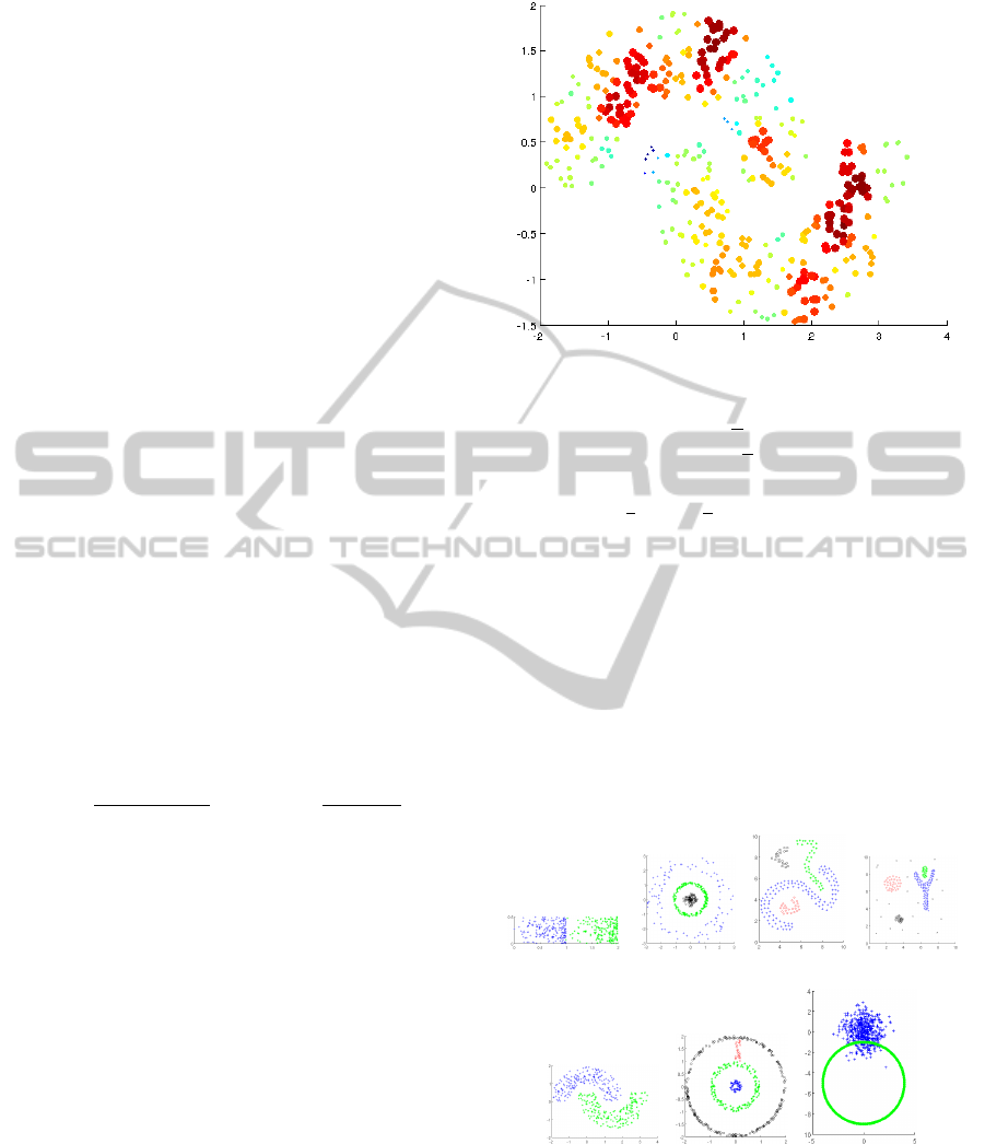
Figure 3 exemplifies the degree of confidence
conf(x
i
) for each data pattern belonging to the Half
Rings data set. Big (and red) points correspond to data
patterns with high confidence, and small (and blue)
points to data patterns with low confidence.
It may be beneficial to the quality of constrained
data clustering choosing only the patterns with more
confidence, less confidence, or a mixture of the two
above, in the RAC and RAL processes instead of us-
ing all the patterns in a data set.
Let X
o
be the ordered set of X in ascend-
ing order of degree of confidence, i.e, X
o
=
{x
o
1
, x
o
2
, ··· , x
o
n
}, conf(x
o
1
) ≤conf(x
o
2
) ≤···≤conf(x
o
n
).
To investigate the previous hypothesis we propose to
apply the RAC and RAL process using a subset X
0
of size m < n of X using one of the following three
criteria:
1. the subset with lowest degree of confidence
(LRAC and LRAL): X
0
= {x
o
1
, ··· , x
o
m
};
2. the subset with highest degree of confidence
(HRAC and HRAL): X
0
= {x
o
n−m+1
, ··· , x
o
n
};
Figure 3: Confidence of each data pattern for Half Rings
data set.
3. the subset of the d
m
2
e patterns with lowest
confidence and the b
m
2
c patterns with high-
est confidence (LHRAC and LHRAL): X
0
=
{x
o
1
, ··· , x
o
d
m
2
e
, , x
o
n−b
m
2
c+1
, ··· , x
o
n
} .
4 EXPERIMENTAL SETUP AND
RESULTS
7 synthetic and 7 real data sets were used to assess
the performance of the proposed approach on a wide
variety of situations, such as data sets with different
cardinality and dimensionality, arbitrary shaped clus-
ters, well separated and touching clusters and distinct
cluster densities.
(a) Bars (b) Circs (c) D2 (d) D3
(e) Half Rings (f) Rings (g) 2 Clusters
Figure 4: Synthetic data sets.
Table 1 presents the summary (number of data
patterns n, number of dimensions d and the number
of data patterns for each cluster) of all data sets
used in our experiments and Figure 4 illustrates
the 2-dimensional synthetic data sets used in our
KDIR2012-InternationalConferenceonKnowledgeDiscoveryandInformationRetrieval
296

Table 1: Data sets overview.
Data sets n d K Cluster Distribution
Bars 400 2 2 2 ×200
Circs 400 2 3 2 ×100 + 200
D2 200 2 4 116 + 39 + 21 + 24
D3 200 2 5 98 + 23 + 23 + 35 + 21
Half Rings 400 2 2 2 ×200
Rings 500 2 4 75 + 150 + 250 + 25
Two Clusters 1000 2 2 2 ×500
Wine 178 13 3 59 + 71 + 48
Yeast Cell 384 17 5 67 + 135 + 75 + 52 + 55
Optdigits 1000 64 10 10 ×100
Iris 150 4 3 3 ×50
House Votes 232 16 2 124 + 108
Breast Cancer 683 9 2 444 + 239
experiments. A brief description for each real
data set is given next. The real data sets used in
our experiments are available at UCI repository
(http://mlearn.ics.uci.edu/MLRepository.html) The
Iris data set consists of 50 patterns from each of
three species of Iris flowers (setosa, virginica and
versicolor) characterized by four features. One of the
clusters is well separated from the other two over-
lapping clusters. Breast Cancer data set is composed
of 683 data patterns characterized by nine features
and divided into two clusters: benign and malignant.
Yeast Cell data set consists of 384 patterns described
by 17 attributes, split into five clusters concerning five
phases of the cell cycle. There are two versions of
this data set, the first one is called Log Yeast and uses
the logarithm of the expression level and the other is
called Std Yeast and is a “standardized” version of the
same data set, with mean 0 and variance 1. Optdigits
is a subset of Handwritten Digits data set containing
only the first 100 objects of each digit, from a total of
3823 data patterns characterized by 64 attributes. The
House Votes data set is composed of two clusters of
votes for each of the U.S. House of Representatives
Congressmen on the 16 key votes identified by the
Congressional Quarterly Almanac. From a total of
435 (267 democrats and 168 republicans) only the
patterns without missing values were considered,
resulting in 232 patterns (125 democrats and 107
republicans). The Wine data set consists of the results
of a chemical analysis of wines grown in the same
region in Italy divided into three clusters with 59, 71
and 48 patterns described by 13 features.
To build the clustering ensembles we used the
k-means clustering algorithm (MacQueen, 1967) to
produce N = 200 data partitions, randomly choos-
ing the number of clusters for each partition from the
set {K
min
, K
min
+ 1, ··· , K
max
−1, K
max
}. The min-
imum and maximum number of clusters were de-
fined as K
min
=

min

2n
20
, max

2n
50
,
√
n

and K
max
=

min

K
min
+ max

2n
50
, 2
√
n

,
n
5

, respectively.
To extract the consensus partition from the co-
association matrix, the average-Link, single-link
(Sneath and Sokal, 1973) and complete-link (Sneath
and Sokal, 1973) were applied for the unconstrained
EAC, while the proposed constrained Average-link al-
gorithm, a constrained version of single-link (Duarte
et al., 2009) and a constrained version of complete-
link (Klein et al., 2002) were used for the constrained
EAC setting. The value of the softness parameter was
set to p = 1. The number of clusters K
∗
of the con-
sensus partitions was defined as the natural number
of clusters K
0
for each data set. To build the sets of
constraints using the RAC process and its variations,
the size of the subset and the number of constraints
was set to m = d0.1ne. For the RAL process and its
variations, the size of the subset (i.e. the size of the
labeled set) was set to m = d0.1ne. Each clustering
combination method was applied 30 times for each
data set.
To evaluate the performance of the combination
methods we used the Consistency index (Ci) (Fred,
2001). Ci measures the fraction of shared data pat-
terns in matching clusters of the consensus partition
(P
∗
) and the real data partition (P
0
) obtained from
ground-truth information. The Consistency index is
computed as
Ci(P
∗
, P
0
) =
1
n
min{K
∗
,K
0
}
∑
k=1
|C
∗
k
∩C
0
k
| (5)
where it is assumed the clusters of P
∗
and P
0
have
been permuted in a way that the cluster C
∗
k
matches
with the real cluster C
0
k
.
Table 2 presents the average Consistency index
(Ci(P
∗
, P
0
) × 100) values for the consensus parti-
tions produced by the clustering combination meth-
ods using RAC process and variations. Column 1
shows the name of the data sets. Columns 2 to
4 (“Unconstrained”) presents the results for the un-
constrained EAC using average-link (AL), single-link
(SL) and complete-link (CL) algorithms. Columns
5 to 16 show the results of the constrained ver-
sion of EAC using RAC, RAL and their variations
for acquiring constraints, respectively, using con-
strained average-link (CAL), constrained single-link
(CSL) and constrained complete-link (CCL) algo-
rithms. It can be seen that the use of constraints usu-
ally (but not always) improves the quality of the con-
sensus partitions. This is more evident when com-
paring the results produced by complete-link with
the ones of constrained complete-link. The cluster-
ing algorithm used for extracting the consensus par-
tition from the co-association matrix (AL, SL, CL,
CAL, CSL and CCL) and constraint acquisition pro-
cess (RAC, LRAC, HRAC, LHRAC, RAL, LRAL,
HRAL and LHRAL) with best performance was con-
EvidenceAccumulationClusteringusingPairwiseConstraints
297

Table 2: Average Consistency index (Ci(P
∗
, P
0
)×100) values for the consensus partitions produced by EAC, and Constrained
EAC using RAC, LRAC, HRAC and LHRAC methods for acquiring constraints.
Acquisition Method Unconstrained RAC LRAC HRAC LHRAC
Extractor Algorithm AL SL CL CAL CSL CCL CAL CSL CCL CAL CSL CCL CAL CSL CCL
Bars 99.15 90.55 54.78 99.83 88.97 85.23 99.85 92.04 64.88 99.85 97.02 67.37 99.93 98.41 67.37
Circs 99.91 100 46.39 99.92 100 87.59 100 100 70.28 99.91 100 66.93 100 100 66.93
D2 73.55 98.3 40.9 79.33 98.3 90.22 76.8 100 86.77 73.55 98.3 88.72 73.35 98.3 88.72
D3 71.62 90.55 46.73 75.2 88.07 53.57 72.95 79.52 40.52 71.75 90.55 39.17 71.48 81.6 39.17
Half Rings 100 100 58.28 100 100 94.16 100 100 76.13 100 100 69.46 100 100 69.46
Rings 74.18 65.05 55.13 76.05 89.19 59.39 77.47 75.63 50.51 74.18 64.12 47.25 74.91 65.73 47.25
Two Clusters 91.06 52.17 51.88 90.69 50.43 68.99 91.35 67.02 57.52 89.36 70.7 55.61 90.75 76.4 55.61
Wine 72.21 72.19 51.39 70.77 56.44 56.93 72.15 58.76 45.28 71.99 67.1 45.21 72.6fire 65.45 45.21
Std Yeast 68.35 47.46 42.55 68.32 39.35 49.25 68.41 42.82 46.54 67.79 47.91 46.05 67.46 46.63 46.05
Optdigits 85.27 61.13 37.43 87.77 60.06 46.28 87.52 62.42 37.27 86.32 62.36 32.16 87.62 64.57 32.16
Log Yeast 42.01 36.52 38.87 41.02 36.43 39.98 41.55 38.06 38.81 41.84 35.76 39.79 41.55 37.41 39.79
Iris 89.93 74.67 72.76 91.27 76.53 72.71 90.22 89.02 47.76 89.8 74.67 49.44 90.76 86 49.44
House Votes 89.25 69.08 53.39 91.01 56.01 72.63 92.41 71.18 67.87 90.22 84.11 73.52 90.85 84.63 73.52
Breast Cancer 96.97 63.01 61.81 96.89 65.03 87.02 96.55 73.69 73.67 96.97 64.19 73.26 96.77 82.96 73.26
Table 3: Average Consistency index (Ci(P
∗
, P
0
)×100) values for the consensus partitions produced by EAC, and Constrained
EAC using RAL, LRAL, HRAL and LHRAL methods for aquiring constraints.
Aquisition Method Unconstrained RAL LRAL HRAL LHRAL
Extractor Algorithm AL SL CL CAL CSL CCL CAL CSL CCL CAL CSL CCL CAL CSL CCL
Bars 99.15 90.55 54.78 99.88 100 76.92 99.95 92.04 65.63 99.15 97.02 69.08 99.27 98.51 68.49
Circs 99.91 100 46.39 100 100 80.64 100 100 67.33 99.91 100 67.5 100 100 66.47
D2 73.55 98.3 40.9 87.67 100 85.35 85.35 100 87.28 73.55 98.3 88.65 74.38 98.3 87.68
D3 71.62 90.55 46.73 79.77 89.82 62.45 76.13 81 43.15 71.75 90.55 37.68 72.62 84.7 43.95
Half Rings 100 100 58.28 100 100 73.23 100 100 56.7 100 100 67.95 100 100 60.58
Rings 74.18 65.05 55.13 84.49 96.01 65.39 81.64 77.93 44.45 74.18 64.12 45.37 77.39 69.37 46.69
Two Clusters 91.06 52.17 51.88 91.76 92.99 61.38 89.18 75.09 60.63 87.17 84.23 64.82 89.54 86.13 66.69
Wine 72.21 72.19 51.39 71.93 67.94 54.18 72.66 51.5 47.77 72.57 68.2 46.55 72.62 61.2 46.61
Std Yeast 68.35 47.46 42.55 69.08 65.59 52.02 69.56 55.63 52.14 64.51 49.93 50.58 67.83 56.67 48.21
Optdigits 85.27 61.13 37.43 92.96 93.71 42.98 91.09 71 39.06 85.41 60.77 33.79 87.64 71.61 36.26
Log Yeast 42.01 36.52 38.87 45.45 59.74 46.7 40.32 45.4 43.12 41.07 37.21 44.06 40.94 45.49 45.1
Iris 89.93 74.67 72.76 93.47 96 56.44 98.33 90.98 49.38 89.93 74.67 49.47 94.09 82.09 49.76
House Votes 89.25 69.08 53.39 90.79 89.93 79.12 93.36 72.14 63.06 89.66 84.11 72.57 91.78 89.77 62.5
Breast Cancer 96.97 63.01 61.81 97.24 95.8 73.74 98.92 79.51 72.98 96.97 64.57 73.63 98.2 85.71 72.99
strained average-link with LRAC, followed by con-
strained average-link again with LHRAC, achieving
the best average Ci results in 5 and 4 out of the 14
data sets, respectively. The complete-link and con-
strained complete-link algorithms never achieved the
best result for any data set. These findings indicate
that constrained average-link is a good constrained
clustering algorithm for producing consensus parti-
tions using the EAC framework, and that acquiring
constraints in a subset of data patterns with low de-
gree of confidence in their assignment to the clusters
lead to an improvement of clustering quality.
Table 3 shows the results for the clustering com-
bination methods using RAL process and variations.
In fact, the unconstrained EAC never achieved a bet-
ter result than the constrained EAC. The best combi-
nation of clustering algorithm and constraint acqui-
sition process was constrained single-link with RAL,
obtaining 8 best results out of 14 data sets, followed
by constrained average with LRAL (again) which
achieved 7 best results out of 14. The success of
constrained single-link with RAL may be explained
by the following facts: constrained single-link is a
hard-constrained algorithm and the number of pair-
wise constraints obtained by using labels is very high
and covers almost all the difficult cluster assignments
in the data set. In this case, if the softness parameter
of constrained average-link have been set to a higher
value, probably its results should have been better. In
fact, the combination of the constrained single-link al-
gorithm with RAL process was the best for the syn-
thetic data sets, obtaining the best results in 6 out
of 7 data sets. Considering only the real data sets,
the combination of the constrained average-link with
LRAL process achieved the best results in 5 out of 7
real data sets. This supports the conclusion that using
the constrained average-link algorithm for extracting
the consensus partition, using the EAC framework,
in conjunction with the LRAL process for acquiring
constraints is a good choice for cluster real data sets.
Once again, the best results were never produced by
the complete-link and constrained complete-link al-
gorithms.
By comparing the results from table 2 with the
ones from table 3 we observe that the RAL process
outperforms RAC. The advantage of using constraints
in clustering combination is also more evident. This
is due to the number of pairwise constraints acquired
by RAL process being significantly higher than the
number of constraints produced by RAC.
5 CONCLUSIONS AND FUTURE
WORK
A new constrained agglomerative hierarchical cluster-
ing algorithm was proposed. It consisted in a modi-
KDIR2012-InternationalConferenceonKnowledgeDiscoveryandInformationRetrieval
298

fication to the average-link clustering algorithm. The
soft-constrained average-link algorithm was applied
in the EAC framework to produce the consensus par-
tition using the co-association matrix as input and out-
performed the hard-constrained clustering algorithms
used for comparison.
The experimental results have shown that con-
strained clustering algorithms usually produce better
consensus partitions than the traditional clustering al-
gorithms, and that acquiring constraints from a subset
of data containing the patterns with the lowest degree
of confidence improves clustering quality.
Future work include the development of an “intel-
ligent” algorithm for acquiring clustering constraints
using the insights gained in this paper, the study of the
effect of the softness parameter, and the establishment
of criteria for its selection.
ACKNOWLEDGEMENTS
This work is supported by FEDER Funds through
the “Programa Operacional Factores de Competitivi-
dade - COMPETE” program and by National Funds
through FCT under the projects FCOMP-01-0124-
FEDER-PEst-OE/EEI/UI0760/2011 and PTDC/EIA -
CCO/103230/2008 and grant SFRH/BD/43785/2008.
REFERENCES
Basu, S. (2005). Semi-supervised clustering: probabilis-
tic models, algorithms and experiments. PhD thesis,
Austin, TX, USA. Supervisor-Mooney, Raymond J.
Basu, S., Davidson, I., and Wagstaff, K. (2008). Con-
strained Clustering: Advances in Algorithms, Theory,
and Applications. Chapman & Hall/CRC.
Davidson, I. and Ravi, S. (2005). Clustering with con-
straints feasibility issues and the k-means algorithm.
In 2005 SIAM International Conference on Data Min-
ing (SDM’05), pages 138–149, Newport Beach,CA.
Domeniconi, C. and Al-Razgan, M. (2009). Weighted clus-
ter ensembles: Methods and analysis. ACM Trans.
Knowl. Discov. Data, 2:17:1–17:40.
Duarte, J. M. M., Fred, A. L. N., and Duarte, F. J. F. (2009).
Combining data clusterings with instance level con-
straints. In Fred, A. L. N., editor, Proceedings of the
9th International Workshop on Pattern Recognition in
Information Systems, pages 49–60. INSTICC PRESS.
Dudoit, S. and Fridlyand, J. (2003). Bagging to Improve the
Accuracy of a Clustering Procedure. Bioinformatics,
19(9):1090–1099.
Fern, X. Z. and Brodley, C. E. (2003). Random projection
for high dimensional data clustering: A cluster ensem-
ble approach. pages 186–193.
Fern, X. Z. and Brodley, C. E. (2004). Solving cluster en-
semble problems by bipartite graph partitioning. In
Proceedings of the twenty-first international confer-
ence on Machine learning, ICML ’04, pages 36–, New
York, NY, USA. ACM.
Fred, A. and Jain, A. (2005). Combining multiple cluster-
ing using evidence accumulation. IEEE Trans Pattern
Analysis and Machine Intelligence, 27(6):835–850.
Fred, A. L. N. (2001). Finding consistent clusters in data
partitions. In Proceedings of the Second International
Workshop on Multiple Classifier Systems, MCS ’01,
pages 309–318, London, UK. Springer-Verlag.
Ge, R., Ester, M., Jin, W., and Davidson, I. (2007).
Constraint-driven clustering. In KDD ’07: Proceed-
ings of the 13th ACM SIGKDD international confer-
ence on Knowledge discovery and data mining, pages
320–329, New York, NY, USA. ACM.
Klein, D., Kamvar, S. D., and Manning, C. D. (2002). From
instance-level constraints to space-level constraints:
Making the most of prior knowledge in data cluster-
ing. In ICML ’02: Proceedings of the Nineteenth In-
ternational Conference on Machine Learning, pages
307–314, San Francisco, CA, USA. Morgan Kauf-
mann Publishers Inc.
MacQueen, J. B. (1967). Some methods for classification
and analysis of multivariate observations. In Cam, L.
M. L. and Neyman, J., editors, Proc. of the fifth Berke-
ley Symposium on Mathematical Statistics and Prob-
ability, volume 1, pages 281–297. University of Cali-
fornia Press.
Sneath, P. and Sokal, R. (1973). Numerical taxonomy. Free-
man, London, UK.
Sokal, R. R. and Michener, C. D. (1958). A statistical
method for evaluating systematic relationships. Uni-
versity of Kansas Scientific Bulletin, 28:1409–1438.
Strehl, A. and Ghosh, J. (2003). Cluster ensembles — a
knowledge reuse framework for combining multiple
partitions. J. Mach. Learn. Res., 3:583–617.
Topchy, A., Jain, A. K., and Punch, W. (2003). Combining
multiple weak clusterings. pages 331–338.
Topchy, A., Minaei-Bidgoli, B., Jain, A. K., and Punch,
W. F. (2004). Adaptive clustering ensembles. In ICPR
’04: Proceedings of the Pattern Recognition, 17th In-
ternational Conference on (ICPR’04) Volume 1, pages
272–275, Washington, DC, USA. IEEE Computer So-
ciety.
Tung, A. K. H., Hou, J., and Han, J. (2000). Coe: Clus-
tering with obstacles entities. a preliminary study. In
PADKK ’00: Proceedings of the 4th Pacific-Asia Con-
ference on Knowledge Discovery and Data Mining,
Current Issues and New Applications, pages 165–168,
London, UK. Springer-Verlag.
Wagstaff, K. L. (2002). Intelligent clustering with instance-
level constraints. PhD thesis, Ithaca, NY, USA. Chair-
Claire Cardie.
Wang, X. and Davidson, I. (2010). Flexible constrained
spectral clustering. In Proceedings of the 16th ACM
SIGKDD international conference on Knowledge dis-
covery and data mining, KDD ’10, pages 563–572,
New York, NY, USA. ACM.
EvidenceAccumulationClusteringusingPairwiseConstraints
299