Improving Toponym Disambiguation

by Iteratively Enhancing Certainty of Extraction

Mena B. Habib and Maurice van Keulen

Faculty of EEMCS, University of Twente, Enschede, The Netherlands

Keywords:

Named Entity Extraction, Named Entity Disambiguation, Uncertain Annotations.

Abstract:

Named entity extraction (NEE) and disambiguation (NED) have received much attention in recent years. Typ-

ical ﬁelds addressing these topics are information retrieval, natural language processing, and semantic web.

This paper addresses two problems with toponym extraction and disambiguation (as a representative example

of named entities). First, almost no existing works examine the extraction and disambiguation interdepen-

dency. Second, existing disambiguation techniques mostly take as input extracted named entities without

considering the uncertainty and imperfection of the extraction process.

It is the aim of this paper to investigate both avenues and to show that explicit handling of the uncertainty

of annotation has much potential for making both extraction and disambiguation more robust. We conducted

experiments with a set of holiday home descriptions with the aim to extract and disambiguate toponyms. We

show that the extraction conﬁdence probabilities are useful in enhancing the effectiveness of disambiguation.

Reciprocally, retraining the extraction models with information automatically derived from the disambigua-

tion results, improves the extraction models. This mutual reinforcement is shown to even have an effect after

several automatic iterations.

1 INTRODUCTION

Named entities are atomic elements in text belong-

ing to predeﬁned categories such as the names of per-

sons, organizations, locations, expressions of times,

quantities, monetary values, percentages, etc. Named

entity extraction (a.k.a. named entity recognition) is

a subtask of information extraction that seeks to lo-

cate and classify those elements in text. This process

has become a basic step of many systems like Infor-

mation Retrieval (IR), Question Answering (QA), and

systems combining these, such as (Habib, 2011).

One major type of named entities is the toponym.

In natural language, toponyms are names used to re-

fer to locations without having to mention the actual

geographic coordinates. The process of toponym ex-

traction (a.k.a. toponym recognition) aims to identify

location names in natural text. The extraction tech-

niques fall into two categories: rule-based or based

on supervised-learning.

Toponym disambiguation (a.k.a. toponym resolu-

tion) is the task of determining which real location is

referred to by a certain instance of a name. Toponyms,

as with named entities in general, are highly ambigu-

ous. For example, according to GeoNames

, the to-

ponym “Paris” refers to more than sixty different ge-

ographic places around the world besides the capital

of France. Figure 1 shows the top ten of the most am-

biguous geographic names. It also shows the long tail

distribution of toponym ambiguity and the percentage

of geographic names with multiple references.

Another source of ambiguousness is that some to-

ponyms are common English words. Table 1 shows

a sample of English-words-like toponyms along with

the number of references they have in the GeoNames

gazetteer.

Table 1: A Sample of English-words-like toponyms.

And 2 The 3

General 3 All 3

In 11 You 11

A 16 As 84

A general principle in our work is our conviction

that Named entity extraction (NEE) and disambigua-

tion (NED) are highly dependent. In previous work

(Habib and van Keulen, 2011), we studied not only

www.geonames.org

399

B. Habib M. and van Keulen M..

Improving Toponym Disambiguation by Iteratively Enhancing Certainty of Extraction.

DOI: 10.5220/0004174903990410

In Proceedings of the International Conference on Knowledge Discovery and Information Retrieval (SSTM-2012), pages 399-410

ISBN: 978-989-8565-29-7

 2012 SCITEPRESS (Science and Technology Publications, Lda.)

1 reference

54%

4 or more

references

29%

12%

2 references

3 references

Figure 1: Toponym ambiguity in GeoNames: top-10, long tail, and reference frequency distribution.

Toponym

Extraction

Direct effect

Toponym

Disambiguation

Reinforcement effect

Figure 2: The reinforcement effect between the toponym

extraction and disambiguation processes.

the positive and negative effect of the extraction pro-

cess on the disambiguation process, but also the po-

tential of using the result of disambiguation to im-

prove extraction. We called this potential for mutual

improvement, the reinforcement effect (see Figure 2).

To examine the reinforcement effect, we con-

ducted experiments on a collection of holiday home

descriptions from the EuroCottage

portal. These de-

scriptions contain general information about the holi-

day home including its location and its neighborhood

(See Figure 4 for an example). As a representative ex-

ample of toponym extraction and disambiguation, we

focused on the task of extracting toponyms from the

description and using them to infer the country where

the holiday property is located.

In general, we concluded that many of the ob-

served problems are caused by an improper treatment

of the inherent ambiguities. Natural language has

the innate property that it is multiply interpretable.

Therefore, none of the processes in information ex-

traction should be ‘all-or-nothing’. In other words,

all steps, including entity recognition, should produce

possible alternatives with associated likelihoods and

dependencies.

In this paper, we focus on this principle. We

turned to statistical approaches for toponym extrac-

tion. The advantage of statistical techniques for ex-

traction is that they provide alternatives for annota-

tions along with conﬁdence probabilities (conﬁdence

for short). Instead of discarding these, as is com-

http://www.eurocottage.com

monly done by selecting the top-most likely candi-

date, we use them to enrich the knowledge for disam-

biguation. The probabilities proved to be useful in en-

hancing the disambiguation process. We believe that

there is much potential in making the inherent uncer-

tainty in information extraction explicit in this way.

For example, phrases like “Lake Como” and “Como”

can be both extracted with different conﬁdence. This

restricts the negative effect of differences in naming

conventions of the gazetteer on the disambiguation

process.

Second, extraction models are inherently imper-

fect and generate imprecise conﬁdence. We were able

to use the disambiguation result to enhance the con-

ﬁdence of true toponyms and reduce the conﬁdence

of false positives. This enhancement of extraction

improves as a consequence the disambiguation (the

aforementioned reinforcement effect). This process

can be repeated iteratively, without any human inter-

ference, as long as there is improvement in the extrac-

tion and disambiguation.

The rest of the paper is organized as follows. Sec-

tion 2 presents related work on NEE and NED. Sec-

tion 3 presents a problem analysis and our general ap-

proach to iterative improvement of toponym extrac-

tion and disambiguation based on uncertain annota-

tions. The adaptations we made to toponym extrac-

tion and disambiguation techniques are described in

Section 4. In Section 5, we describe the experimen-

tal setup, present its results, and discuss some obser-

vations and their consequences. Finally, conclusions

and future work are presented in Section 6.

2 RELATED WORK

NEE and NED are two areas of research that are well-

covered in literature. Many approaches were devel-

oped for each. NEE research focuses on improving

KDIR2012-InternationalConferenceonKnowledgeDiscoveryandInformationRetrieval

400

the quality of recognizing entity names in unstruc-

tured natural text. NED research focuses on improv-

ing the effectiveness of determining the actual entities

these names refer to. As mentioned earlier, we focus

on toponyms as a subcategory of named entities. Is

this section, we brieﬂy survey a few major approaches

for toponym extraction and disambiguation.

2.1 Named Entity Extraction

NEE is a subtask of Information Extraction (IE) that

aims to annotate phrases in text with its entity type

such as names (e.g., person, organization or loca-

tion name), or numeric expressions (e.g., time, date,

money or percentage). The term ‘named entity recog-

nition (extraction)’ was ﬁrst mentioned in 1996 at the

Sixth Message Understanding Conference (MUC-6)

(Grishman and Sundheim, 1996), however the ﬁeld

started much earlier. The vast majority of proposed

approaches for NEE fall in two categories: hand-

made rule-based systems and supervised learning-

based systems.

One of the earliest rule-based system is FASTUS

(Hobbs et al., 1993). It is a nondeterministic ﬁnite

state automaton text understanding system used for

IE. In the ﬁrst stage of its processing, names and

other ﬁxed form expressions are recognized by em-

ploying specialized microgrammars for short, multi-

word ﬁxed phrases and proper names. Another ap-

proach for NEE is matching against pre-speciﬁed

gazetteers such as done in LaSIE (Gaizauskas et al.,

1995; Humphreys et al., 1998). It looks for single

and multi-word matches in multiple domain-speciﬁc

full name (locations, organizations, etc.) and key-

word lists (company designators, person ﬁrst names,

etc.). It supports hand-coded grammar rules that make

use of part of speech tags, semantic tags added in the

gazetteer lookup stage, and if necessary the lexical

items themselves. The idea behind supervised learn-

ing is to discover discriminative features of named en-

tities by applying machine learning on positive and

negative examples taken from large collections of an-

notated texts. The aim is to automatically generate

rules that recognize instances of a certain category en-

tity type based on their features. Supervised learning

techniques applied in NEE include Hidden Markov

Models (HMM) (Zhou and Su, 2002), Decision Trees

(Sekine, 1998), Maximum Entropy Models (Borth-

wick et al., 1998), Support Vector Machines (Isozaki

and Kazawa, 2002), and Conditional Random Fields

(CRF) (McCallum and Li, 2003)(Finkel et al., 2005).

Imprecision in information extraction is expected,

especially in unstructured text where a lot of noise ex-

ists. There is an increasing research interest in more

formally handling the uncertainty of the extraction

process so that the answers of queries can be asso-

ciated with correctness indicators. Only recently have

information extraction and probabilistic database re-

search been combined for this cause (Gupta, 2006).

Imprecision in information extraction can be rep-

resented by associating each extracted ﬁeld with a

probability value. Other methods extend this ap-

proach to output multiple possible extractions instead

of a single extraction. It is easy to extend probabilis-

tic models like HMM and CRF to return the k high-

est probability extractions instead of a single most

likely one and store them in a probabilistic database

(Michelakis et al., 2009). Managing uncertainty in

rule-based approaches is more difﬁcult than in statis-

tical ones. In rule-based systems, each rule is asso-

ciated with a precision value that indicates the per-

centage of cases where the action associated with that

rule is correct. However, there is little work on main-

taining probabilities when the extraction is based on

many rules, or when the ﬁrings of multiple rules over-

lap. Within this context, (Michelakis et al., 2009)

presents a probabilistic framework for managing the

uncertainty in rule-based information extraction sys-

tems where the uncertainty arises due to the varying

precision associated with each rule by producing ac-

curate estimates of probabilities for the extracted an-

notations. They also capture the interaction between

the different rules, as well as the compositional nature

of the rules.

2.2 Toponym Disambiguation

According to (Wacholder et al., 1997), there are dif-

ferent kinds of toponym ambiguity. One type is struc-

tural ambiguity, where the structure of the tokens

forming the name are ambiguous (e.g., is the word

“Lake” part of the toponym “Lake Como” or not?).

Another type of ambiguity is semantic ambiguity,

where the type of the entity being referred to is am-

biguous (e.g., is “Paris” a toponym or a girl’s name?).

A third form of toponym ambiguity is reference am-

biguity, where it is unclear to which of several alter-

natives the toponym actually refers (e.g., does “Lon-

don” refer to “London, UK” or to “London, Ontario,

Canada”?). In this work, we focus on the structural

and the reference ambiguities.

Toponym reference disambiguation or resolution

is a form of Word Sense Disambiguation (WSD).

According to (Buscaldi and Rosso, 2008), existing

methods for toponym disambiguation can be clas-

siﬁed into three categories: (i) map-based: meth-

ods that use an explicit representation of places on a

map; (ii) knowledge-based: methods that use external

ImprovingToponymDisambiguationbyIterativelyEnhancingCertaintyofExtraction

401

knowledge sources such as gazetteers, ontologies, or

Wikipedia; and (iii) data-driven or supervised: meth-

ods that are based on machine learning techniques.

An example of a map-based approach is (Smith and

Crane, 2001), which aggregates all references for all

toponyms in the text onto a grid with weights repre-

senting the number of times they appear. References

with a distance more than two times the standard de-

viation away from the centroid of the name are dis-

carded.

Knowledge-based approaches are based on the hy-

pothesis that toponyms appearing together in text are

related to each other, and that this relation can be

extracted from gazetteers and knowledge bases like

Wikipedia. Following this hypothesis, (Rauch et al.,

2003) used a toponym’s local linguistic context to de-

termine the toponym type (e.g., river, mountain, city)

and then ﬁltered out irrelevant references by this type.

Another example of a knowledge-based approach is

(Overell and Ruger, 2006) which uses Wikipedia to

generate co-occurrence models for toponym disam-

biguation.

Supervised learning approaches use machine

learning techniques for disambiguation. (Smith and

Mann, 2003) trained a naive Bayes classiﬁer on to-

ponyms with disambiguating cues such as “Nashville,

Tennessee” or “Springﬁeld, Massachusetts”, and

tested it on texts without these clues. Similarly, (Mar-

tins et al., 2010) used Hidden Markov Models to an-

notate toponyms and then applied Support Vector Ma-

chines to rank possible disambiguations.

In this paper, we chose to use HMM and CRF to

build statistical models for extraction. We developed

a clustering-based approach for the toponym disam-

biguation task. This is described in Section 4.

3 PROBLEM ANALYSIS AND

GENERAL APPROACH

The task we focus on is to extract toponyms from Eu-

roCottage holiday home descriptions and use them to

infer the country where the holiday property is lo-

cated. We use this country inference task as a rep-

resentative example of disambiguating extracted to-

ponyms.

Our initial results from our previous work, where

we developed a set of hand-coded grammar rules to

extract toponyms, showed that effectiveness of dis-

ambiguation is affected by the effectiveness of ex-

traction. We also proved the feasibility of a reverse

inﬂuence, namely how the disambiguation result can

be used to improve extraction by ﬁltering out terms

found to be highly ambiguous during disambiguation.

Training

data

Extraction model

(here: HMM & CRF)

learning

Test

data

extraction

Matching

(here: with GeoNames)

Disambiguation

(here: country inference)

extracted

toponyms

candidate

entities

including

alternatives

with probabilities

Result

highly ambiguous terms

and false positives

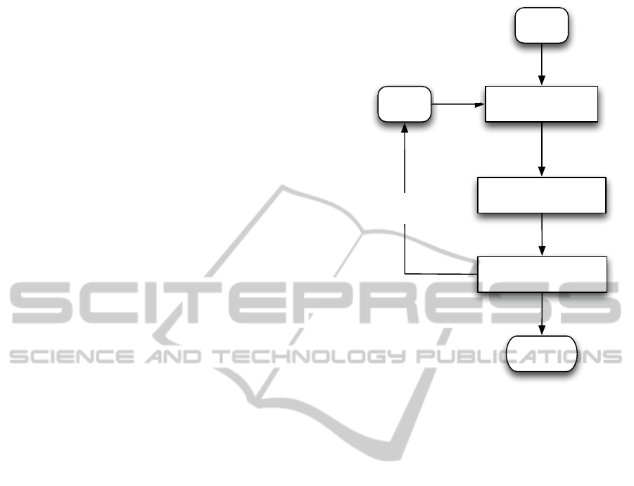
Figure 3: General approach.

One major problem with the hand-coded gram-

mar rules is its “All-or-nothing” behavior. One can

only annotate either “Lake Como” or “Como”, but

not both. Furthermore, hand-coded rules don’t pro-

vide extraction conﬁdences which we believe to be

useful for the disambiguation process. We therefore

propose an entity extraction and disambiguation ap-

proach based on uncertain annotations. The general

approach illustrated in Figure 3 has the following

steps:

1. Prepare training data by manually annotating

named entities (in our case toponyms) appearing

in a subset of documents of sufﬁcient size.

2. Use the training data to build a statistical extrac-

tion model.

3. Apply the extraction model on test data and train-

ing data. Note that we explicitly allow uncertain

and alternative annotations with probabilities.

4. Match the extracted named entities against one or

more gazetteers.

5. Use the toponym entity candidates for the disam-

biguation process (in our case we try to disam-

biguate the country of the holiday home descrip-

tion).

6. Evaluate the extraction and disambiguation re-

sults for the training data and determine a list of

highly ambiguous named entities and false posi-

tives that affect the disambiguation results. Use

them to re-train the extraction model.

KDIR2012-InternationalConferenceonKnowledgeDiscoveryandInformationRetrieval

402

7. The steps from 2 to 6 are repeated automatically

until there is no improvement any more in either

the extraction or the disambiguation.

Note that the reason for including the training data

in the process, is to be able to determine false pos-

itives in the result. From test data one cannot deter-

mine a term to be a false positive, but only to be highly

ambiguous.

4 OUR APPROACHES

In this section we illustrate the selected techniques for

the extraction and disambiguation processes. We also

present our adaptations to enhance the disambigua-

tion by handling uncertainty and the imperfection in

the extraction process, and how the extraction and dis-

ambiguation processes can reinforce each other itera-

tively.

4.1 Toponym Extraction

For toponym extraction, we trained two statistical

named entity extraction modules

, one based on Hid-

den Markov Models (HMM) and one based on Con-

ditional Ramdom Fields (CRF).

4.1.1 HMM Extraction Module

The goal of HMM is to ﬁnd the optimal tag se-

quence T = t

, t

, ..., t

for a given word sequence

W = w

, w

, ..., w

that maximizes:

P(T |W ) =

P(T )P(W | T )

P(W )

(1)

where P(W ) is the same for all candidate tag se-

quences. P(T ) is the probability of the named entity

(NE) tag. It can be calculated by Markov assumption

which states that the probability of a tag depends only

on a ﬁxed number of previous NE tags. Here, in this

work, we used n = 4. So, the probability of a NE tag

depends on three previous tags, and then we have,

P(T ) = P(t

) ×P(t

, t

)

×P(t

, t

) ×. . . ×P(t

n−3

, t

n−2

, t

n−1

) (2)

As the relation between a word and its tag depends

on the context of the word, the probability of the cur-

rent word depends on the tag of the previous word and

the tag to be assigned to the current word. So P(W |T )

We made use of the lingpipe toolkit for development:

http://alias-i.com/lingpipe

can be calculated as:

P(W |T ) = P(w

) ×P(w

, t

)×

. . . ×P(w

n−1

, t

) (3)

The prior probability P(t

i−3

, t

i−2

, t

i−1

) and the

likelihood probability P(w

) can be estimated from

training data. The optimal sequence of tags can be

efﬁciently found using the Viterbi dynamic program-

ming algorithm (Viterbi, 1967).

4.1.2 CRF Extraction Module

HMMs have difﬁculty with modeling overlapped,

non-independent features of the output part-of-speech

tag of the word, the surrounding words, and capital-

ization patterns. Conditional Random Fields (CRF)

can model these overlapping, non-independent fea-

tures (Wallach, 2004). Here we used a linear chain

CRF, the simplest model of CRF.

A linear chain Conditional Random Field deﬁnes

the conditional probability:

P(T |W ) =

exp



∑

i=1

∑

j=1

i−1

, t

, W, i)



∑

t,w

exp



∑

i=1

∑

j=1

i−1

, t

, W, i)



(4)

where f is set of m feature functions, λ

is the weight

for feature function f

, and the denominator is a nor-

malization factor that ensures the distribution p sums

to 1. This normalization factor is called the parti-

tion function. The outer summation of the partition

function is over the exponentially many possible as-

signments to t and w. For this reason, computing the

partition function is intractable in general, but much

work exists on how to approximate it (Sutton and Mc-

Callum, 2011).

The feature functions are the main components

of CRF. The general form of a feature function is

i−1

, t

, W, i), which looks at tag sequence T , the

input sequence W , and the current location in the se-

quence (i).

We used the following set of features for the pre-

vious w

i−1

, the current w

, and the next word w

i+1

• The tag of the word.

• The position of the word in the sentence.

• The normalization of the word.

• The part of speech tag of the word.

• The shape of the word (Capitalization/Small state,

Digits/Characters, etc.).

• The sufﬁx and the preﬁx of the word.

An example for a feature function which pro-

duces a binary value for the current word shape is

Capitalized:

i−1

, t

, W, i) =



1 if w

is Capitalized

0 otherwise

(5)

ImprovingToponymDisambiguationbyIterativelyEnhancingCertaintyofExtraction

403

The training process involves ﬁnding the optimal

values for the parameters λ

that maximize the condi-

tional probability P(T | W ). The standard parameter

learning approach is to compute the stochastic gradi-

ent descent of the log of the objective function:

∂

∂λ

∑

i=1

log p(t

)) −

∑

j=1

2σ

(6)

where the term

∑

j=1

2σ

is a Gaussian prior on λ to

regularize the training. In our experiments we used

the prior variance σ

=4. The rest of the derivation for

the gradient descent of the objective function can be

found in (Wallach, 2004).

4.1.3 Extraction Modes of Operation

We used the extraction models to retrieve sets of an-

notations in two ways:

• First-Best. In this method, we only consider the

ﬁrst most likely set of annotations that maximizes

the probability P(T |W ) for the whole text. This

method does not assign a probability for each

individual annotation, but only to the whole re-

trieved set of annotations.

• N-Best. This method returns a top-N of possible

alternative hypotheses in order of their estimated

likelihoods p(t

). The conﬁdence scores are as-

sumed to be conditional probabilities of the anno-

tation given an input token. A very low cut-off

probability is additionally applied as well. In our

experiments, we retrieved the top-25 possible an-

notations for each document with a cut-off proba-

bility of 0.1.

4.2 Toponym Disambiguation

For the toponym disambiguation task, we only select

those toponyms annotated by the extraction models

that match a reference in GeoNames. We furthermore

use a clustering-based approach to disambiguate to

which entity an extracted toponym actually refers.

4.2.1 The Clustering Approach

The clustering approach is an unsupervised disam-

biguation approach based on the assumption that to-

ponyms appearing in same document are likely to re-

fer to locations close to each other distance-wise. For

our holiday home descriptions, it appears quite safe

to assume this. For each toponym t

, we have, in gen-

eral, multiple entity candidates. Let R(t

) = {r

∈

GeoNames gazetteer} be the set of reference candi-

dates for toponym t

. Additionally each reference r

in GeoNames belongs to a country Country

. By tak-

ing one entity candidate for each toponym, we form

a cluster. A cluster, hence, is a possible combination

of entity candidates, or in other words, one possible

entity candidate of the toponyms in the text. In this

approach, we consider all possible clusters, compute

the average distance between the candidate locations

in the cluster, and choose the cluster Cluster

min

with

the lowest average distance. We choose the most of-

ten occurring country in Cluster

min

for disambiguat-

ing the country of the document. In effect the above-

mentioned assumption states that the entities that be-

long to Cluster

min

are the true representative entities

for the corresponding toponyms as they appeared in

the text. Equations 7 through 11 show the steps of the

described disambiguation procedure.

Clusters = {{r

, r

, . . . , r

} |

∀t

∈ d •r

∈ R(t

)} (7)

Cluster

min

= argmin

Cluster

∈Clusters

average distance of

Cluster

(8)

Countries

min

= {Country

| r

∈ Cluster

min

∧r

∈ Country

}

(9)

Country

winner

= argmax

Country

∈Countries

min

freq(Country

)

(10)

where

freq(Country

) =

∑

i=1



1 if r

∈ Country

0 otherwise

(11)

4.2.2 Handling Uncertainty of Annotations

Equation 11 gives equal weights to all toponyms. The

countries of toponyms with a very low extraction con-

ﬁdence probability are treated equally to toponyms

with high conﬁdence; both count fully. We can take

the uncertainty in the extraction process into account

by adapting Equation 11 to include the conﬁdence of

the extracted toponyms.

freq(Country

) =

∑

i=1



p(t

) if r

∈ Country

0 otherwise

(12)

In this way terms which are more likely to be to-

ponyms have a higher contribution in determining the

country of the document than less likely ones.

KDIR2012-InternationalConferenceonKnowledgeDiscoveryandInformationRetrieval

404

4.3 Improving Certainty of Extraction

In the abovementioned improvement, we make use of

the extraction conﬁdence to help the disambiguation

to be more robust. However, those probabilities are

not accurate and reliable all the time. Some extraction

models (like HMM in our experiments) retrieve some

false positive toponyms with high conﬁdence proba-

bilities. Moreover, some of these false positives have

many entity candidates in many countries according

to GeoNames (e.g., the term “Bar” refers to 58 differ-

ent locations in GeoNames in 25 different countries;

see Figure 7). These false positives affect the disam-

biguation process.

This is where we take advantage of the reinforce-

ment effect. To be more precise, we introduce an-

other class in the extraction model called ‘highly am-

biguous’ and annotate those terms in the training set

with this class that (1) are not manually annotated as

a toponym already, (2) have a match in GeoNames,

and (3) the disambiguation process ﬁnds more than τ

countries for documents that contain this term, i.e.,



{c | ∃d •t

∈ d ∧c = Country

winner

for d}



≥τ (13)

The threshold τ can be experimentally and automat-

ically determined (see Section 5.3). The extraction

model is subsequently re-trained and the whole pro-

cess is repeated without any human interference as

long as there is improvement in extraction and disam-

biguation process for the training set. Observe that

terms manually annotated as toponym stay annotated

as toponyms. Only terms not manually annotated as

toponym but for which the extraction model predicts

that they are a toponym anyway, are affected. The

intention is that the extraction model learns to avoid

prediction of certain terms to be toponyms when they

appear to have a confusing effect on the disambigua-

tion.

5 EXPERIMENTAL RESULTS

In this section, we present the results of experiments

with the presented methods of extraction and disam-

biguation applied to a collection of holiday properties

descriptions. The goal of the experiments is to inves-

tigate the inﬂuence of using annotation conﬁdence on

the disambiguation effectiveness. Another goal is to

show how to automatically improve the imperfect ex-

traction model using the outcomes of the disambigua-

tion process and subsequently improving the disam-

biguation also.

2-room apartment 55 m2: living/dining room with

1 sofa bed and satellite-TV, exit to the balcony. 1

room with 2 beds (90 cm, length 190 cm). Open

kitchen (4 hotplates, freezer). Bath/bidet/WC.

Electric heating. Balcony 8 m2. Facilities: tele-

phone, safe (extra). Terrace Club: Holiday com-

plex, 3 storeys, built in 1995 2.5 km from the

centre of Armacao de Pera, in a quiet position.

For shared use: garden, swimming pool (25 x

12 m, 01.04.-30.09.), paddling pool, children’s

playground. In the house: reception, restaurant.

Laundry (extra). Linen change weekly. Room

cleaning 4 times per week. Public parking on

the road. Railway station ”Alcantarilha” 10 km.

Please note: There are more similar properties for

rent in this same residence. Reception is open

16 hours (0800-2400 hrs). Lounge and reading

room, games room. Daily entertainment for adults

and children. Bar-swimming pool open in sum-

mer. Restaurant with Take Away service. Break-

fast buffet, lunch and dinner(to be paid for sepa-

rately, on site). Trips arranged, entrance to water

parks. Car hire. Electric cafetiere to be requested

in adavance. Beach football pitch. IMPORTANT:

access to the internet in the computer room (ex-

tra). The closest beach (350 m) is the ”Sehora

da Rocha”, Playa de Armacao de Pera 2.5 km.

Please note: the urbanisation comprises of eight 4

storey buildings, no lift, with a total of 185 apart-

ments. Bus station in Armacao de Pera 4 km.

Figure 4: An example of a EuroCottage holiday home de-

scription (toponyms in bold).

5.1 Data Set

The data set we use for our experiments is a collection

of traveling agent holiday property descriptions from

the EuroCottage portal. The descriptions not only

contain information about the property itself and its

facilities, but also a description of its location, neigh-

boring cities and opportunities for sightseeing. The

data set includes the country of each property which

we use to validate our results. Figure 4 shows an ex-

ample for a holiday property description. The manu-

ally annotated toponyms are written in bold.

The data set consists of 1579 property descriptions

for which we constructed a ground truth by manually

annotating all toponyms. We used the collection in

our experiments in two ways:

• Train Test Set. We split the data set into a train-

ing set and a validation test set with ratio 2 : 1,

and used the training set for building the extrac-

tion models and ﬁnding the highly ambiguous to-

ponyms, and the test set for a validation of ex-

ImprovingToponymDisambiguationbyIterativelyEnhancingCertaintyofExtraction

405

bath shop terrace shower at

house the all in as

they here to table garage

parking and oven air gallery

each a farm sauna sandy

(a) Sample of false positive toponyms extracted by HMM.

north zoo west well travel

tram town tower sun sport

(b) Sample of false positive toponyms extracted by CRF.

Figure 5: False positive extracted toponyms.

traction and disambiguation effectiveness against

“new and unseen” data.

• All Train Set. We used the whole collection as

a training and test set for validating the extraction

and the disambiguation results.

The reason behind using the All Train set for

traing and testing is that the size of the collection is

considered small for NLP tasks. We want to show

that the results of the Train Test set can be better if

there is enough training data.

5.2 Experiment 1: Effect of Extraction

with Conﬁdence Probabilities

The goal of this experiment is to evaluate the effect

of allowing uncertainty in the extracted toponyms on

the disambiguation results. Both a HMM and a CRF

extraction model were trained and evaluated in the

two aforementioned ways. Both modes of operation

(First-Best and N-Best) were used for inferring the

country of the holiday descriptions as described in

Section 4.2. We used the unmodiﬁed version of the

clustering approach (Equation 11) with the output of

First-Best method, while we used the modiﬁed ver-

sion (Equation 12) with the output of N-Best method

to make use of the conﬁdence probabilities assigned

to the extracted toponyms.

Results are shown in Table 2. It shows the per-

centage of holiday home descriptions for which the

correct country was successfully inferred.

We can clearly see that the N-Best method outper-

forms the First-Best method for both the HMM and

the CRF models. This supports our claim that dealing

with alternatives along with their conﬁdences yields

better results.

5.3 Experiment 2: Effect of Extraction

Certainty Enhancement

While examining the results of extraction for both

Table 2: Effectiveness of the disambiguation process for

First-Best and N-Best methods in the extraction phase.

(a) On Train Test set

HMM CRF

First-Best 62.59% 62.84%

N-Best 68.95% 68.19%

(b) On All Train set

HMM CRF

First-Best 70.7% 70.53%

N-Best 74.68% 73.32%

Table 3: Effectiveness of the disambiguation process using

manual annotations.

Train Test set All Train set

79.28% 78.03%

HMM and CRF, we discovered that there were many

false positives among the extracted toponyms, i.e.,

words extracted as a toponym and having a reference

in GeoNames, that are in fact not toponyms. Samples

of such words are shown in Figures 5(a) and 5(b).

These words affect the disambiguation result, if the

matching entities in GeoNames belong to many dif-

ferent countries.

We applied the proposed technique introduced in

Section 4.3 to reinforce the extraction conﬁdence of

true toponyms and to reduce them for highly ambigu-

ous false positive ones. We used the N-Best method

for extraction and the modiﬁed clustering approach

for disambiguation. The best threshold τ for annotat-

ing terms as highly ambiguous has been experimen-

tally determined (see section 5.3).

Table 3 shows the results of the disambiguation

process using the manually annotated toponyms. Ta-

ble 5 show the extraction results using the state of the

art Stanford named entity recognition model

. Stan-

ford is a NEE system based on CRF model which

incorporates long-distance information (Finkel et al.,

2005). It achieves good performance consistently

across different domains. Tables 4 and 6 show the ef-

fectiveness of the disambiguation and the extraction

processes respectively along iterations of reﬁnement.

The “No Filtering” rows show the initial results of

disambiguation and extraction before any reﬁnements

have been done.

We can see an improvement in HMM extraction

and disambiguation results. It starts with lower ex-

traction effectiveness than Stanford model but it out-

performs after retraining the model. This support our

claim that the reinforcement effect can help imper-

fect extraction models iteratively. Further analysis

and discussion shown in Section 5.5.

http://nlp.stanford.edu/software/CRF-NER.shtml

KDIR2012-InternationalConferenceonKnowledgeDiscoveryandInformationRetrieval

406

0.3

0.4

0.5

0.6

0.7

0.8

0.9

140

No Filt.

Threshold

Recall

Precision

(a) HMM 1st iteration.

0.77

0.78

0.79

0.8

0.81

2 3 4 5 6 7 8 9 10 11 12 14 19 21 25 28 47 48 58 No

Filt.

Threshold

Recall

Precision

(b) HMM 2nd iteration.

0.77

0.78

0.79

0.8

0.81

0.82

0.83

0.84

No Filt.

Threshold

Recall

Precision

0.55

0.6

0.65

0.7

0.75

0.8

2 3 4 5 6 7 8 9 10 12 14 15 17 18 24 25 28 35 45 55 No

Filt.

Threshold

Recall

Precision

(d) CRF 1st iteration.

Figure 6: The ﬁltering threshold effect on the extraction effectiveness (On All Train set)

Table 4: Effectiveness of the disambiguation process after

iterative reﬁnement.

(a) On Train Test set

HMM CRF

No Filtering 68.95% 68.19%

1st Iteration 73.28% 68.44%

2nd Iteration 73.53% 68.44%

3rd Iteration 73.53% -

(b) On All Train set

HMM CRF

No Filtering 74.68% 73.32%

1st Iteration 77.56% 73.32%

2nd Iteration 78.57% -

3rd Iteration 77.55% -

Table 5: Effectiveness of the extraction using Stanford

NER.

(a) On Train Test set

Pre. Rec. F1

Stanford NER 0.8385 0.4374 0.5749

(b) On All Train set

Pre. Rec. F1

Stanford NER 0.8622 0.4365 0.5796

5.4 Experiment 3: Optimal Cutting

Threshold

Figures 6(a), 6(b), 6(c) and 6(d) show the effec-

tiveness of the HMM and CRF extraction models

Table 6: Effectiveness of the extraction process after itera-

tive reﬁnement.

(a) On Train Test set

HMM

Pre. Rec. F1

No Filtering 0.3584 0.8517 0.5045

1st Iteration 0.7667 0.5987 0.6724

2nd Iteration 0.7733 0.5961 0.6732

3rd Iteration 0.7736 0.5958 0.6732

CRF

No Filtering 0.6969 0.7136 0.7051

1st Iteration 0.6989 0.7131 0.7059

2nd Iteration 0.6989 0.7131 0.7059

3rd Iteration - - -

(b) On All Train set

HMM

Pre. Rec. F1

No Filtering 0.3751 0.9640 0.5400

1st Iteration 0.7808 0.7979 0.7893

2nd Iteration 0.7915 0.7937 0.7926

3rd Iteration 0.8389 0.7742 0.8053

CRF

No Filtering 0.7496 0.7444 0.7470

1st Iteration 0.7496 0.7444 0.7470

2nd Iteration - - -

3rd Iteration - - -

ImprovingToponymDisambiguationbyIterativelyEnhancingCertaintyofExtraction

407

at ﬁrst iteration in terms of Precision, Recall, and

F1 measures versus the possible thresholds τ. Note

that the graphs need to be read from right to left; a

lower threshold means more terms being annotated as

highly ambiguous. At the far right, no terms are an-

notated as such anymore, hence this is equivalent to

no ﬁltering.

We select the threshold with the highest F1 value.

For example, the best threshold value is 3 in ﬁgure

6(a). Observe that for HMM, the F1 measure (from

right to left) increases, hence a threshold is chosen

that improves the extraction effectiveness. It does not

do so for CRF, which is prominent cause for the poor

improvements we saw earlier for CRF.

5.5 Further Analysis and Discussion

For deep analysis of results, we present in Table 7

detailed results for the property description shown in

Figure 4. We have the following observations and

thoughts:

• From table 2, we can observe that both HMM

and CRF initial models were improved by consid-

ering conﬁdence of the extracted toponyms (see

Section 5.2). However, for HMM, still many

false positives were extracted with high conﬁ-

dence scores in the initial extraction model.

• The initial HMM results showed a very high recall

rate with a very low precision. In spite of this our

approach managed to improve precision signiﬁ-

cantly through iterations of reﬁnement. The re-

ﬁnement process is based on removing highly am-

biguous toponyms resulting in a slight decrease in

recall and an increase in precision. In contrast,

CRF started with high precision which could not

be improved by the reﬁnement process. Appar-

ently, the CRF approach already aims at achieving

high precision at the expense of some recall (see

Table 6).

• In table 6 we can see that the precision of the

HMM outperforms the precision of CRF after it-

erations of reﬁnement. This results in achieving

better disambiguation results for the HMM over

the CRF (see Table 4)

• It can be observed that the highest improvement

is achieved on the ﬁrst iteration. This where most

of the false positives and highly ambiguous to-

ponyms are detected and ﬁltered out. In the subse-

quent iterations, only few new highly ambiguous

These graphs are supposed to be discrete, but we

present it like this to show the trend of extraction effective-

ness against different possible cutting thresholds.

toponyms appeared and were ﬁltered out (see Ta-

ble 6).

• It can be seen in Table 7 that initially non-

toponym phrases like “.-30.09.)” and “IMPOR-

TANT” were falsely extracted by HMM. These

don’t have a GeoNames reference, so were not

considered in the disambiguation step, nor in the

subsequent re-training. Nevertheless they dis-

appeared from the top-N annotations. The rea-

son for this behavior is that initially the extrac-

tion models were trained on annotating for only

one type (toponym), whereas in subsequent itera-

tions they were trained on two types (toponym and

‘highly ambiguous non-toponym’). Even though

the aforementioned phrases were not included in

the re-training, their conﬁdences still fell below

the 0.1 cut-off threshold after the 1st iteration.

Furthermore, after one iteration the top-25 anno-

tations contained 4 toponym and 21 highly am-

biguous annotations.

6 CONCLUSIONS AND FUTURE

WORK

NEE and NED are inherently imperfect processes that

moreover depend on each other. The aim of this pa-

per is to examine and make use of this dependency for

the purpose of improving the disambiguation by iter-

atively enhancing the effectiveness of extraction, and

vice versa. We call this mutual improvement, the re-

inforcement effect. Experiments were conducted with

a set of holiday home descriptions with the aim to ex-

tract and disambiguate toponyms as a representative

example of named entities. HMM and CRF statistical

approaches were applied for extraction. We compared

extraction in two modes, First-Best and N-Best. A

clustering approach for disambiguation was applied

with the purpose to infer the country of the holiday

home from the description.

We examined how handling the uncertainty of ex-

traction inﬂuences the effectiveness of disambigua-

tion, and reciprocally, how the result of disambigua-

tion can be used to improve the effectiveness of ex-

traction. The extraction models are automatically re-

trained after discovering highly ambiguous false pos-

itives among the extracted toponyms. This iterative

process improves the precision of the extraction. We

argue that our approach that is based on uncertain an-

notation has much potential for making information

extraction more robust against ambiguous situations

and allowing it to gradually learn. We provide insight

into how and why the approach works by means of an

KDIR2012-InternationalConferenceonKnowledgeDiscoveryandInformationRetrieval

408

Table 7: Deep analysis for the extraction process of the property shown in Figure 4 (∈: present in GeoNames; #refs: number

of references; #ctrs: number of countries).

GeoNames lookup Conﬁdence Disambiguation

Extracted Toponyms ∈ #refs #ctrs probability result

Manually

annotated

toponyms

Armacao de Pera

√

1 1 -

Correctly

Classiﬁed

Alcantarilha

√

1 1 -

Sehora da Rocha × - - -

Playa de Armacao de Pera × - - -

Armacao de Pera

√

1 1 -

Initial HMM

model with

First-Best

extraction

method

Balcony 8 m2 × - - -

Misclassiﬁed

Terrace Club

√

1 1 -

Armacao de Pera

√

1 1 -

.-30.09.) × - - -

Alcantarilha

√

1 1 -

Lounge

√

2 2 -

Bar

√

58 25 -

Car hire × - - -

IMPORTANT × - - -

Sehora da Rocha × - - -

Playa de Armacao de Pera × - - -

Bus

√

15 9 -

Armacao de Pera

√

1 1 -

Initial HMM

model with

N-Best

extraction

method

Alcantarilha

√

1 1 1

Correctly

Classiﬁed

Sehora da Rocha × - - 1

Armacao de Pera

√

1 1 1

Playa de Armacao de Pera × - - 0.999849891

Bar

√

58 25 0.993387918

Bus

√

15 9 0.989665883

Armacao de Pera

√

1 1 0.96097006

IMPORTANT × - - 0.957129986

Lounge

√

2 2 0.916074183

Balcony 8 m2 × - - 0.877332628

Car hire × - - 0.797357377

Terrace Club

√

1 1 0.760384949

√

11 9 0.455276943

.-30.09.) × - - 0.397836259

.-30.09. × - - 0.368135755

. × - - 0.358238066

. Car hire × - - 0.165877044

adavance. × - - 0.161051997

HMM model after

iteration with

N-Best extraction

method

Alcantarilha

√

1 1 0.999999999

Correctly

Classiﬁed

Sehora da Rocha × - - 0.999999914

Armacao de Pera

√

1 1 0.999998522

Playa de Armacao de Pera × - - 0.999932808

Initial CRF

model with

First-Best

extraction

method

Armacao × - - -

Correctly

Classiﬁed

Pera

√

2 1 -

Alcantarilha

√

1 1 -

Sehora da Rocha × - - -

Playa de Armacao de Pera × - - -

Armacao de Pera

√

1 1 -

Initial CRF

model with

N-Best

extraction

method

Alcantarilha

√

1 1 0.999312439

Correctly

Classiﬁed

Armacao × - - 0.962067016

Pera

√

2 1 0.602834683

Trips

√

3 2 0.305478198

Bus

√

15 9 0.167311005

Lounge

√

2 2 0.133111374

Reception

√

1 1 0.105567287

ImprovingToponymDisambiguationbyIterativelyEnhancingCertaintyofExtraction

409

in-depth analysis of what happens to individual cases

during the process.

We claim that this approach can be adapted to suit

any kind of named entities. It is just required to de-

velop a mechanism to ﬁnd highly ambiguous false

positives among the extracted named entities. Co-

herency measures can be used to ﬁnd highly ambigu-

ous named entities. For future research, we plan to

apply and enhance our approach for other types of

named entities and other domains. Furthermore, the

approach appears to be fully language independent,

therefore we like to prove that this is the case and

investigate its effect on texts in multiple and mixed

languages.

REFERENCES

Borthwick, A., Sterling, J., Agichtein, E., and Grishman, R.

(1998). NYU: Description of the MENE named entity

system as used in MUC-7. In Proc. of MUC-7.

Buscaldi, D. and Rosso, P. (2008). A conceptual density-

based approach for the disambiguation of toponyms.

Int’l Journal of Geographical Information Science,

22(3):301–313.

Finkel, J. R., Grenager, T., and Manning, C. (2005). ncorpo-

rating non-local information into information extrac-

tion systems by gibbs sampling. In roceedings of the

43nd Annual Meeting of the Association for Compu-

tational Linguistics, ACL 2005, pages 363–370.

Gaizauskas, R., Wakao, T., Humphreys, K., Cunningham,

H., and Wilks, Y. (1995). University of Shefﬁeld: De-

scription of the LaSIE system as used for MUC-6. In

Proc. of MUC-6, pages 207–220.

Grishman, R. and Sundheim, B. (1996). Message under-

standing conference - 6: A brief history. In Proc. of

Int’l Conf. on Computational Linguistics, pages 466–

471.

Gupta, R. (2006). Creating probabilistic databases from in-

formation extraction models. In VLDB, pages 965–

976.

Habib, M. B. (2011). Neogeography: The challenge of

channelling large and ill-behaved data streams. In

Workshops Proc. of the 27th ICDE 2011, pages 284–

287.

Habib, M. B. and van Keulen, M. (2011). Named entity

extraction and disambiguation: The reinforcement ef-

fect. In Proc. of MUD 2011, Seatle, USA, pages 9–16.

Hobbs, J., Appelt, D., Bear, J., Israel, D., Kameyama, M.,

Stickel, M., and Tyson, M. (1993). Fastus: A system

for extracting information from text. In Proc. of Hu-

man Language Technology, pages 133–137.

Humphreys, K., Gaizauskas, R., Azzam, S., Huyck, C.,

Mitchell, B., Cunningham, H., and Wilks, Y. (1998).

University of Shefﬁeld: Description of the Lasie-II

system as used for MUC-7. In Proc. of MUC-7.

Isozaki, H. and Kazawa, H. (2002). Efﬁcient support vector

classiﬁers for named entity recognition. In Proc. of

COLING 2002, pages 1–7.

Martins, B., Anast

acio, I., and Calado, P. (2010). A ma-

chine learning approach for resolving place references

in text. In Proc. of AGILE 2010.

McCallum, A. and Li, W. (2003). Early results for named

entity recognition with conditional random ﬁelds, fea-

ture induction and web-enhanced lexicons. In Proc. of

CoNLL 2003, pages 188–191.

Michelakis, E., Krishnamurthy, R., Haas, P. J., and

Vaithyanathan, S. (2009). Uncertainty management

in rule-based information extraction systems. In Pro-

ceedings of the 35th SIGMOD international confer-

ence on Management of data, SIGMOD ’09, pages

101–114, New York, NY, USA. ACM.

Overell, J. and Ruger, S. (2006). Place disambiguation with

co-occurrence models. In Proc. of CLEF 2006.

Rauch, E., Bukatin, M., and Baker, K. (2003). A

conﬁdence-based framework for disambiguating geo-

graphic terms. In Workshop Proc. of the HLT-NAACL

2003, pages 50–54.

Sekine, S. (1998). NYU: Description of the Japanese NE

system used for MET-2. In Proc. of MUC-7.

Smith, D. and Crane, G. (2001). Disambiguating ge-

ographic names in a historical digital library. In

Research and Advanced Technology for Digital Li-

braries, volume 2163 of LNCS, pages 127–136.

Smith, D. and Mann, G. (2003). Bootstrapping toponym

classiﬁers. In Workshop Proc. of HLT-NAACL 2003,

pages 45–49.

Sutton, C. and McCallum, A. (2011). An introduction to

conditional random ﬁelds. Foundations and Trends in

Machine Learning. To appear.

Viterbi, A. (1967). Error bounds for convolutional codes

and an asymptotically optimum decoding algorithm.

Information Theory, IEEE Transactions on, 13(2):260

– 269.

Wacholder, N., Ravin, Y., and Choi, M. (1997). Disam-

biguation of proper names in text. In Proc. of ANLC

1997, pages 202–208.

Wallach, H. (2004). Conditional random ﬁelds: An in-

troduction. Technical Report MS-CIS-04-21, Depart-

ment of Computer and Information Science, Univer-

sity of Pennsylvania.

Zhou, G. and Su, J. (2002). Named entity recognition using

an hmm-based chunk tagger. In Proc. ACL2002, pages

473–480.

KDIR2012-InternationalConferenceonKnowledgeDiscoveryandInformationRetrieval

410