
On the Evolvability of Different Computational Architectures
using a Common Developmental Genome
Konstantinos Antonakopoulos and Gunnar Tufte
Department of Computer and Information Science, Norwegian University of Science and Technology,
Sem Sælandsvei 7-9, NO-7491, Trondheim, Norway
Keywords:
Genetic Representation, Cellular Automata, Boolean Network, L-systems, Evolvability.
Abstract:
Artificial organisms comprise a method that enables the construction of complex systems with structural and/or
computational properties. In this work we investigate whether a common developmental genome can favor
the evolvability of different computational architectures. This is rather interesting, especially when limited
computational resources is the case. The commonly evolved genome showed ability to boost the evolvability of
the different computational architectures requiring fewer resources and in some cases, finding better solutions.
1 INTRODUCTION
Artificial systems often target organisms or systems
with some kind of functionality. Target functional-
ity may include systems aiming to solve problems, be
it structural (Steiner et al., 2009), or computational
(Harding et al., 2007). In the first case, the target is
the structure itself. In the second case, the target is a
functionality given by the computational function of
the nodes and their connections.
Targeting problems with a structural versus a com-
putational goal is quite different. Most EvoDevo (i.e.,
Evolutionary Developmental) systems consist of a
genotype targeting special phenotypic structures (i.e.,
structures that comprise connected computational ele-
ments) - even when the target is a computational func-
tion. The structural property of the phenotype may re-
duce the solution efficiency or even the computational
goal that can be achieved.
To be able to develop such phenotypic structures,
there is a need to further understand the properties of
the targeted computational architectures. An analysis
of the possibilities and constraints involved in the de-
velopment of various computational architectures, fo-
cusing on the form, functionality and the inherent bio-
logical properties, was presented in (Antonakopoulos
and Tufte, 2009). The architectures studied therein
were Boolean Networks (BN) (Kauffman, 1993), Ar-
tificial Neural Networks (ANN) (Astor and Adami,
2000), Cellular Automata (CA) (Tufte and Haddow,
2005), and Cellular Neural Networks (CNN) (Chua
and Yang, 1988). The common property of these arc-
hitectures is that they are considered as sparsely-
connected networks. This common property moti-
vates a further investigation on how a mapping pro-
cess can work on a class of architectures in a more
general way towards complex problems. This is elab-
orated by examining how universal properties and
processes can be included in a development mapping,
through an EvoDevo approach (Robert, 2004).
In biology, a specie is often used as a basic unit
for biological classification and for taxonomic rank-
ing. Species are individuals sharing the same genetic,
developmental and ecological processes (Wilkins,
2010). Inspired by multicellularity and the organ-
isms’ ability to exploit different developmental paths
based on environmental factors, we explored the po-
tentiality of using the same developmental mapping to
develop not a specific, but different classes of archi-
tectures (i.e., species), using a common genetic repre-
sentation (Antonakopoulos and Tufte, 2011).
The hypothesis for this work is to see whether
common developmental genomes can prove benefi-
cial over developmental genomes evolved for each
specie, separately, towards complex computations. To
see if the hypothesis holds, two things should be fur-
ther investigated. First, whether the same mapping
(i.e., a common developmental genome), can favor
the evolvability of different computational architec-
tures under the same environment when resources are
limited. Second, if the same developmental mapping
can favor the evolvability of different computational
architectures (i.e., CA and BN), with a focus in prob-
lems of increasing complexity. Only then, we will
122
Antonakopoulos K. and Tufte G..
On the Evolvability of Different Computational Architectures using a Common Developmental Genome.
DOI: 10.5220/0004176501220129
In Proceedings of the 4th International Joint Conference on Computational Intelligence (ECTA-2012), pages 122-129
ISBN: 978-989-8565-33-4
Copyright
c
2012 SCITEPRESS (Science and Technology Publications, Lda.)

have concrete evidence for our hypothesis.
The first step mentioned above, comprise also the
motivation of this work. The second step will be ex-
amined and published elsewhere. Here, we are study-
ing the same computational architectures (i.e., CA
and BN), as different species. The computational ar-
chitectures in this setup will have limited computa-
tional resources to evolve. It is of interest then to
investigate whether common developmental genomes
can favor the evolvability of these architectures, as op-
posed to genomes evolved separately for each archi-
tecture.
The rest of the article is laid out as follows. Sec-
tion 2 addresses the challenges involved in such a de-
velopmental model. The common genetic representa-
tion is given at section 3. Experiments come in sec-
tion 4 with the conclusion and future work in section
5.
2 DEVELOPMENT FOR
SPARSELY-CONNECTED
COMPUTATIONAL
STRUCTURES
The developmental goal is to be able to generate
not a specific, but different classes of structures (i.e.,
species), using the same developmental model. This
should be achieved through the same developmental
approach. Such developmental approach requires suf-
ficient knowledge of the targeted computational archi-
tectures and of their governing properties. That is,
for the 2-dimensional CA, the properties of dimen-
sionality and neighborhood must be defined, where
the connectivity is predetermined (i.e., the Euclidean
space). For boolean networks, the connectivity (i.e.,
the node connections of the network), must be deter-
mined. The problem just described can be better ex-
pressed as three-challenge problem: (a) the genome
challenge, (b) the developmental processes involved
in the model, and (c) the developmental model chal-
lenge.
2.1 The Genome Challenge
Based on the properties of a 2D-CA, the genome con-
tains information about the cells at each developmen-
tal step, in order to place them on a 2D-CA lattice
structure. The wiring of the cell is given by the CA’s
neighborhood. At the same time and based on the
properties of a boolean network, the genome contains
enough information to feed the developmental model
to develop a boolean network, at each developmental
step.
2.2 The Developmental Processes
Challenge
The resulting structure is able to grow, alter the func-
tionality of a cell/node, and shrink. These processes
are introduced in the developmental mapping through
growth, differentiation, and apoptosis (i.e., the death
of the cell/node). Having these properties in mind,
our genome incorporates the notion of chromosomes
- inspired by biology. Each chromosome contains re-
spective information about the structural and/or func-
tional requirements. More specifically, a chromosome
will contain the information required for the cell/node
creation (i.e., for the CAs and BNs), where another
chromosome will contain the information required for
wiring the nodes (i.e., for BNs). The notion of chro-
mosomes allows us to exploit the genome in a mod-
ular way in the sense that if an additional computa-
tional architecture need to be described through the
same genome, more chromosomes can be added to it.
2.3 The Developmental Model
Challenge
The developmental model is able to develop these
structures, taking into account the special properties
employed by each architecture. The developmental
model receives the same genome as input, regardless
of the target architecture. Then, it is possible – de-
pending on some properties of the genome – to dis-
criminate whether it will develop a CA or a BN.
3 THE COMMON GENETIC
REPRESENTATION
In biology, a specie is often used as the basic unit for
biological classification and for taxonomic ranking.
As such, an organism with unifying properties and
same characteristics can be of the same specie. Figure
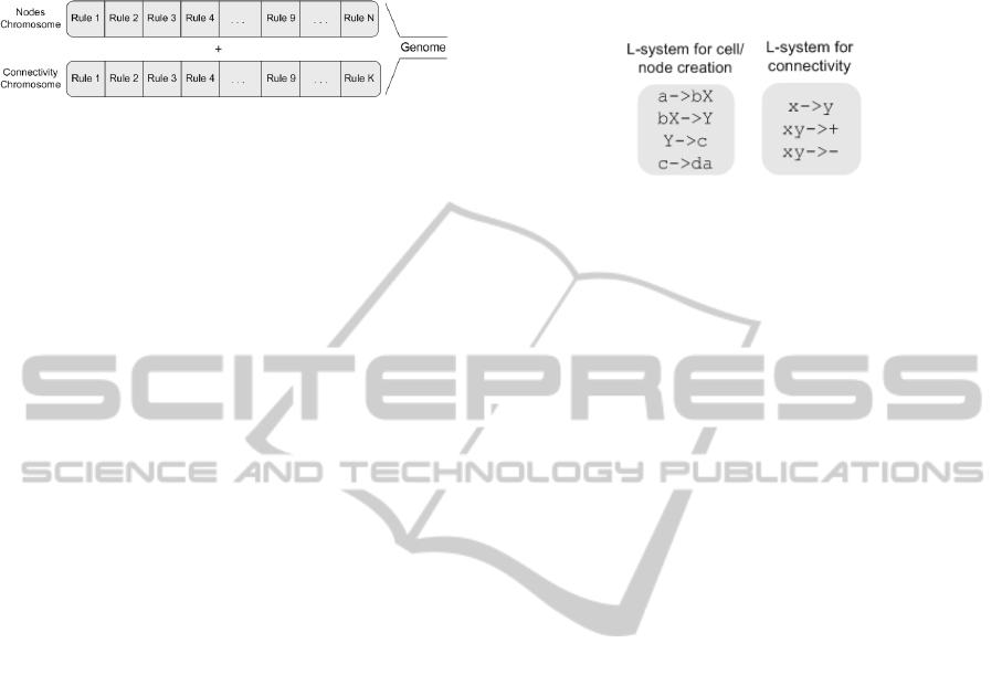
1, show how the genome looks like. The genome is
split into two parts (chromosomes). The first chromo-
some is responsible for creating the cells/nodes. The
second chromosome is responsible for creating the
connectivity (i.e., for the BNs). Each chromosome
is built out of rules. Each rule has sufficient infor-
mation for cell/node creation and connectivity. Also,
the rules are of certain length. Those destined for
cell/node creation are different from the ones for con-
OntheEvolvabilityofDifferentComputationalArchitecturesusingaCommonDevelopmentalGenome
123
nectivity. Consequently, chromosomes contain differ-
ent rules.
Figure 1: This is how the genome looks like with the
genome split into two (chromosomes). The first chromo-
some is responsible for generating the cells/nodes whereas
the second chromosome is responsible for generating the
connectivity of the network.
3.1 An L-system for the Genetic
Representation
A rewriting approach was chosen due to the ease of
defining specific rule set, that can target to rewrite
specific features of a structure, e.g., connections or
node functions that enable a way of splitting genetic
information into separate information carrying units
(i.e., chromosomes).
A prominent model is L-systems. They are rewrit-
ing grammars, able to describe developmental sys-
tems, simulate biological processes (Lindenmayer
and Prusinkiewicz, 1989), and describe computa-
tional machines (Staffer and Sipper, 1998). Since
there are different types of rules in the two chromo-
somes, there is a need for separate L-systems. The
first L-system processes the rules of the first chromo-
some, while the second L-system deals with the con-
nectivity rules of the second chromosome.
3.2 The L-system for the First
Chromosome
The L-system used here is context-sensitive. As such,
development is using the strict predecessor/ancestor
to determine the applicable production rule. The rules
are able to incorporate all the cell processes. Table
1(a), shows the type of symbols used by the L-system
of the first chromosome. Some cells perform special
cell processes and influence the intermediate and fi-
nal phenotypes. Symbol a is the axiom. Apart from
the symbols a, b, and c, which perform growth of
the phenotype, symbol d performs apoptosis, leading
to the deletion of the current rule (i.e., cell/node), of
the intermediate phenotype. Additionally, symbols X
and Y, are responsible for differentiation, leading to
the replacement of the predecessor cell/node (i.e., if
X→Y the outcome will be Y, whereas, if Y→X the out-
come will be X). For the shake of simplicity, the length
of each rule is 4 symbols (i.e., 4x8bits=32bits).
For node/cell generation the L-system runs for 100
timesteps and then stops. As such, the intermediate
phenotypes generated by development are of variable
size.
(a) (b)
Figure 2: (a) Example of L-system rules for the first chro-
mosome, (b) Example of L-system rules for the second
chromosome.
Figure 2(a), gives an example of a L-system for
the first chromosome. A simple example with step-
by-step development of a 2D-CA architecture is illus-
trated at figure 3. Development starts with the axiom
(a) representing a cell at developmental step (DS) 0.
Since the axiom is found in the L-system rules, de-
velopment continues and the next rule triggered is the
a→bX. This rule will create two more cells b and X,
resulting in growth of the CA, at DS 1. The next rule
triggered is bX→Y. Since X→Y denotes differentia-
tion, the symbol X is replaced by Y, at DS 2. For differ-
entiation to occur, the rules should either be X→Y or
Y→X. Next, rule Y→c triggers causing again growth
of the CA, at DS 3. At DS 4, the rule c→da is trig-
gered causing the death of the cell c and the growth of
the CA with the cell a. From DS 5 up to DS 8, rules
are being triggered once more in the same sequence.
3.3 The L-system for the Second
Chromosome
The rules are able to generate the connections neces-
sary for the wiring of the nodes. They contain sym-
bols which when executed by the L-system, result in
creating a connection forward or backwards from the
current node. Each node in the network has unique
numbering; the current node has always the number
zero and any nodes starting from the current node for-
ward have positive numbering, where nodes that exist
from the current node backwards, have negative num-
bering. So, there is a need to differentiate between
the current and the next node, using different symbols
and also whether a connection will be created forward
or backward from the current node.
The rules involved in connectivity are not as com-
plex as those of first chromosome. The length of the
rules here is also 4 symbols / rule. Also, there is a
need to assure that the chromosome will have suf-
ficient information for the developmental processes
IJCCI2012-InternationalJointConferenceonComputationalIntelligence
124
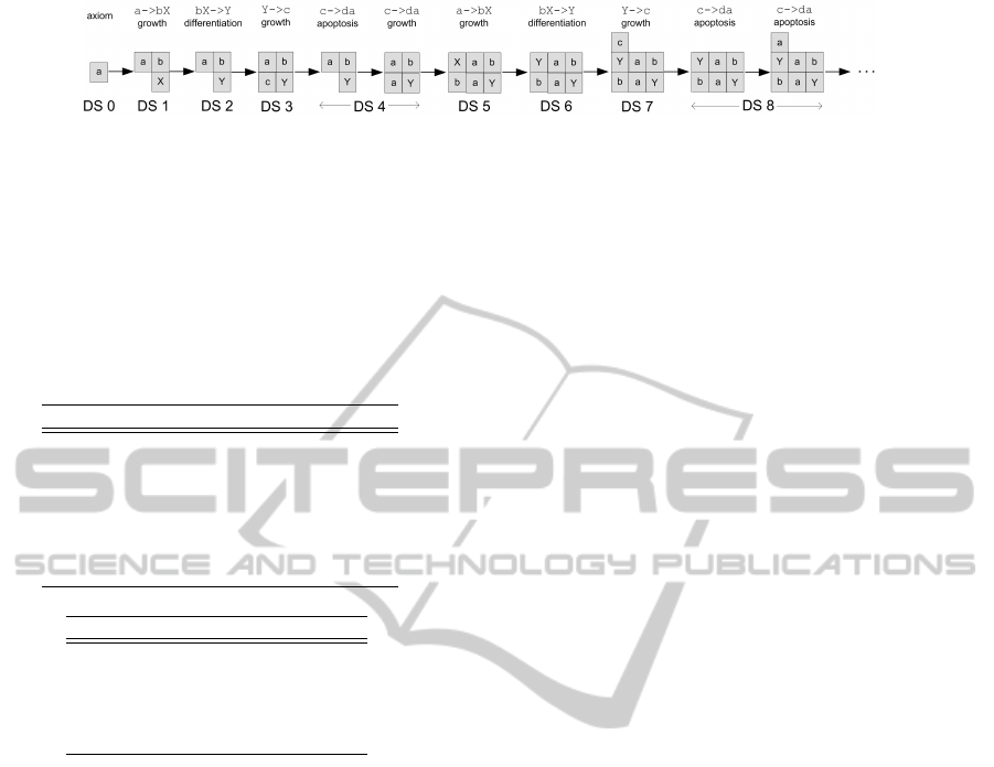
Figure 3: A step-by-step development of a 2D-CA architecture based on the example L-system for the first chromosome.
(i.e., growth, differentiation and apoptosis). The L-
system uses is a D0L (i.e., with zero-sided interac-
tions). An example L-system for the second chromo-
some is shown at figure 2(b), and the symbols used
are explained at Table 1(b).
Table 1: (a) Symbol table for Node generation, (b) Symbol
table for Connectivity generation.
(a)
Symbol Description
a (AXIOM) Add (growth)
b Add (growth)
c Add (growth)
d Delete (apoptosis)
X Substitute (differentiation)
Y Substitute (differentiation)
→ Production
(b)
Symbol Description
x Node (different from y)
y Node (different from x)
+ Connect forward
– Connect backwards
→ Production
The axiom rule for the second chromosome is
x→y. It means that development initially searches if
the axiom exists. If so, development continues and
looks for rules of type xy→+value or xy→-value.
In short, these two rules imply that if two different
(i.e., distinct) nodes are found (x6=y), then it creates
a connection forward (if the rule includes a ’+’), or
backwards (if the rule includes a ’-’). The field value
is encoded in the genotype and denotes the node num-
ber for the generated connection. For example, rule
xy→+3 denotes that a connection will be created from
the current node (node 0), to the one being three nodes
forward. Similarly, rule xy→-3 denotes that a con-
nection will be created starting from the current node
(node 0), to the one that is three nodes backwards. If
value=0, a self-connection is created to the current
node. A step-by-step development of a boolean net-
work based on the chromosomes of Table 1(a) and
1(b), can be found at (Antonakopoulos and Tufte,
2011) and is not shown here due to page limitation.
The modularity of the genome, gives the possibility
to development itself to enable or disable parts of it
(chromosomes), when this is required and driven by
the goal set. For example, if the target architecture is
a 2D-CA, the second chromosome (i.e., connectivity)
is disabled, since connectivity is predetermined. Sim-
ilarly for BN development, both chromosomes are en-
abled (i.e., nodes and connectivity).
3.4 The Genetic Algorithm for the
Common Genetic Representation
A genetic algorithm is used to generate and evolve the
rules found in the genome (i.e., in the chromosomes).
Since there are two separate L-systems involved in
development, the evolutionary process comprise two
phases: node and connectivity generation. Mutation
and single-point crossover were used as genetic op-
erators. Mutation may happen anywhere inside the 4-
symbol rule, ensuring that the production symbol (→)
is not distorted by mutation. That is, we want to make
sure that after mutation, the production symbol still
exists in the rule (i.e., the rule is valid). Single-point
crossover is performed at the location of the produc-
tion symbol, ensuring that a valid rule is created as
offspring. The evolutionary cycle ends after a prede-
termined number of generations.
4 EXPERIMENTS
In (Antonakopoulos and Tufte, 2011), we investigated
the ability of the representation to evolve different
computational architectures using a structured-based
fitness. Here we study the ability of our representation
to deal with problems using a computational fitness;
we take an experimental approach using the same ge-
netic representation on both architectures (CA and
BN), towards sufficient solutions when: i. a sepa-
rately genome is evolved for each of the architecture,
and ii. a common genome is evolved for architectures
altogether.
4.1 Experimental Setup
We use a total number of 36 rules for node genera-
tion and for connectivity (i.e., 32x36=1152bits). It
is important to note that a rule can be reused during
development. Development runs for 100 timesteps for
each individual. The evaluation of the phenotypes for
OntheEvolvabilityofDifferentComputationalArchitecturesusingaCommonDevelopmentalGenome
125

the CA and the BN is given by the cell types of Table
2.
Table 2: Cell types and their functionality.
Cell Type Function name
a NAND
b OR
c AND
d IDENTITY CELL
X XOR
Y NOT
A 6x6 2D-CA and a N = 36 BN is used. The rea-
son is that the two architectures must to be compara-
ble; have the same state space (i.e., 2
36
). The number
of outgoing connections per node is K = 5. For more
than 5 inputs/node, a self-connection to the originat-
ing node is created instead. Generational mixing was
used as global selection mechanism and Rank selec-
tion for parental selection. Unless otherwise stated,
mutation rate was set to .0005 and crossover rate to
.001.
4.2 Search for Cycle Attractors
Using the experimental setup described in section 4.1,
we run a set of 10 experiments of 5000 generations
each. For each individual, a random initial state was
created and fed into the architecture. The fitness func-
tion gives credit for cycle attractors between 2-21; the
best score is assigned for cycle attractors of size 11.
Figure 4(a) shows the average fitness plots over
the 10 runs for genomes evolved separately. The BN
managed to find sufficiently good solutions using a
large amount of available resources (Rsep
BN
). The
CA found also rather good solutions, needing less
than half of the available resources (Rsep
CA
).
The average fitness plot over the 10 runs for com-
monly evolved genomes is shown at figure 4(b). In
this case, genomes were able to find reasonable solu-
tions. The BN achieved a max average of 70% fitness
using half of the available resources (Rcom
BN
), where
the CA achieved a fitness of 68%, acquiring almost
all of the resources (Rcom
CA
).
4.3 Search for Transient Phase and
Attractors
Using the same setup, we also run a set of 10 exper-
iments of 5000 generations each. For each individ-
ual, a random initial state was created and fed into
the architecture. The fitness function gives credit for
transients with a maximum size of 10 after which an
attractor of maximum size of 20 must follow. Point
(a)
(b)
Figure 4: Cycle Attractor experiment: (a) Averaged fitness
plot for the different architectures with genomes evolved
separately, (b) Averaged fitness plot for different architec-
tures with a commonly evolved genome.
attractors are also being taken into account (cycles of
1). The transient phase has a range between 1-10 (best
score is assigned for transients of size 5), where at-
tractors have a range between 1-21 (best score is as-
signed for attractors of size 11). Both fitness param-
eters (i.e., transient phase and attractors) are normal-
ized into half and their partial scores were summed to
give the final score.
Figure 5(a) shows the average fitness plot over 10
runs for genomes evolved separately. The CA was
able to find a sufficient solution, requiring a large
amount of resources (Rsep
CA
). The BN was able to
find only fair solutions acquiring more than half of
the resources available (Rsep
BN
).
In the case of the commonly evolved genome of
figure 5(b), both architectures were able to achieve
similar performance as previously, but consumed sig-
nificantly less resources. The CA reached a max
average fitness of 86% at generation 800 (Rcom
CA
),
where the BN reached a 55% fitness at generation
1750 (Rcom
BN
).
IJCCI2012-InternationalJointConferenceonComputationalIntelligence
126
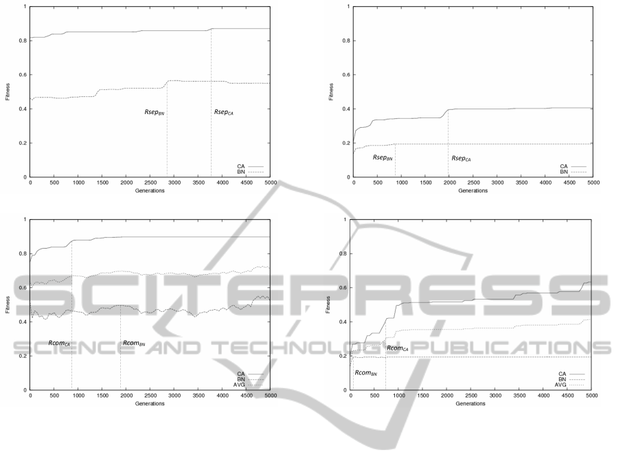
(a)
(b)
Figure 5: Transient with attractors experiment: (a) Av-
eraged fitness plot for the different architectures with
genomes evolved separately, (b) Averaged fitness plot for
different architectures with a commonly evolved genome.
4.4 Synchronization Task
For this task, the goal is to find a CA that given any
initial configuration s within M time steps, reaches
a final configuration that oscillates between all zeros
and all ones on successive time steps. M, the desired
upper bound on the synchronization time, is a param-
eter of the task that depends on the lattice size (Das
et al., 1995). Here, we relaxed the rule of all ones
and all zeros by introducing a synchronization thresh-
old. It means that we may have configurations of ze-
ros or ones up to the threshold limit. In this case, this
threshold is set to 80%. This implies that configura-
tions filled up with 80% zeros or ones are eligible as
target configurations. Here, a 1D-CA and a BN of
size 36 is used, with the mutation rate being .002 and
the crossover rate .001. Each individual is developed
for 1000 timesteps.
Figure 6(a) shows the average fitness plot over
10 runs for the separately evolved genomes case.
The CA was able to achieve a max average fitness
of 40% at generation 2000 (Rsep
CA
), where the BN
(a)
(b)
Figure 6: Synchronization task experiment: (a) Averaged
fitness plot for the different architectures with genomes
evolved separately, (b) Averaged fitness plot for different
architectures with a commonly evolved genome.
gave moderate solutions (18%) at generation 850
(Rsep
BN
).
In the case of commonly evolved genomes at fig-
ure 6(b), both architectures needed fewer resources to
achieve the same results as in the separately evolved
genome case. As such, the CA reached the same
fitness at generation 750 (Rcom
CA
), where the BN
reached the fitness of 18% at generation 90 (Rcom
BN
).
In addition to that, the commonly evolved genome
achieved better overall fitness; the CA reached an av-
erage of 60% and the BN an average of 20% (for the
total of the available resources).
5 CONCLUSIONS AND FUTURE
WORK
In this work, we investigated whether and when
commonly evolved genomes favor the evolvability
of different computational architectures, as opposed
to genomes evolved separately for each architecture.
The computational architectures targeted herein were
OntheEvolvabilityofDifferentComputationalArchitecturesusingaCommonDevelopmentalGenome
127

a 6x6 non-uniform 2D-CA and a BN of size N = 36
and were considered as different species. In addition,
the different genome cases evolved in a setup with
only limited computational resources.
The search for a cycle attractor problem showed
that the common genome was not able to show favor-
able results for the development of the architectures.
The separately evolved genome was able to give par-
tially better results; the CA was able to evolve requir-
ing less than half of the resources available.In the case
of transient phase and attractor search, both genome
cases ended up with a similar fitness performance but
the commonly evolved genome consumed consider-
ably fewer resources. In the synchronization task
problem, the commonly evolved genome was able to
evolve the architectures acquiring again less resources
than in the separately evolved genome case.
The construction of a common genome able to de-
velop different computational architectures proved to
be beneficial. There are cases where resources are
not infinitely available or not available at the given
moment. Artificial organisms need to have ways to
overcome such problems if they are to continue to
evolve at all (much like in the nature). Commonly
evolved genomes boosted the evolvability of the ar-
chitectures. In two of the experiments we studied,
it required considerably fewer resources than in the
case of the genome evolved separately. The reason
behind the superiority of the common developmental
genomes is somewhat intuitive. Common genomes in
this configuration, involve two fitness functions (i.e.,
one for node generation and another for connectivity),
defining a set of optimal solutions over each evolu-
tionary cycle. So, we can say that the nodes genome
stands as an ideal source of information for the con-
nectivity genome and ultimately, the development of
the phenotypes.
But there is more to that. It may be that common
developmental genomes are more amenable to devel-
opmental drive (Arthur, 2001). Or, they may have a
positive influence in directing evolution and pushing
the developmental system in phenotypic directions
where it would have been impossible to achieve with
ordinary genomes (i.e., genomes evolved separately
for each architecture at hand). The latter is identi-
fied as developmental bias (Raff, 2000). To conclude,
more research needs to be done towards the identi-
fication of: i. potential relations between mutation
and selection in the underlying genetic process, and
ii. inherent ontogenetic directionalities (i.e., dynam-
ics) for common developmental genomes, during the
stages of evolution.
Closing, the notion of chromosomes in our repre-
sentation, allows us to exploit the genome in a modu-
lar way in a sense that if additional computational ar-
chitectures need to be incorporated in the future and
expressed by the same genome, more chromosomes
can be attached. Changing the way of looking into the
architectures, i.e., instead of looking at them as dif-
ferent species, we could consider them as organs of
a common developing biological entity. That brings
up a case where architectures need to be merged (as
is the case in biological organs). Since the overall
goal of this work is to target more adaptive scalable
systems able of complex computation, the exploration
of these merged computational architectures (i.e., hy-
brid architectures) with the same genome and devel-
opmental model but even further, the ability to shape
the phenotype of our system (phenotypic shaping) as
modules in order to change the dynamic properties of
the entire system, paves the way for promising future
research.
REFERENCES
Antonakopoulos, K. and Tufte, G. (2009). Possibilities and
constraints of basic computational units in develop-
mental systems. In Norsk Informatikkonferanse, NIK-
2009, pages 73–84.
Antonakopoulos, K. and Tufte, G. (2011). A common
genetic representation capable of developing distinct
computational architectures. In IEEE Congress on
Evolutionary Computation (CEC), pages 1264–1271.
Arthur, W. (2001). Developmental drive: an important
determinant of the direction of phenotypic evolution.
Evolution & Development, 3(4):271–278.
Astor, J. C. and Adami, C. (2000). A developmental model
for the evolution of artificial neural networks. Artifi-
cial Life, 6(3):189–218.
Chua, L. and Yang, L. (1988). Cellular neural networks:
theory. IEEE Transactions on Circuits and Systems,
35(10):1257–1272.
Das, R., Crutchfield, J. P., Mitchell, M., and Hanson, J. E.
(1995). Evolving globally synchronized cellular au-
tomata. In Eshelman, L. J., editor, Proceedings of
the Sixth International Conference on Genetic Algo-
rithms, pages 336–343. Morgan Kaufmann Publishers
Inc.
Harding, S. L., Miller, J. F., and Banzhaf, W. (2007).
Self-modifying cartesian genetic programming. In
GECCO ’07: Proceedings of the 9th annual confer-
ence on Genetic and evolutionary computation, pages
1021–1028, New York, NY, USA. ACM.
Kauffman, S. A. (1993). The Origins of Order. Oxford
University Press.
Lindenmayer, A. and Prusinkiewicz, P. (1989). Develop-
mental models of multicellular organisms: A com-
puter graphics perspective. In Langton, C. G., edi-
tor, Artificial Life: Proceedings of an Interdisciplinary
Workshop on the Synthesis and Simulation of Living
IJCCI2012-InternationalJointConferenceonComputationalIntelligence
128

Systems, pages 221–249. Addison-Wesley Publishing
Company.
Raff, R. (2000). Evo-devo: The evolution of a new disci-
pline. Nature Reviews in Genetics, 1:74–79.
Robert, J. S. (2004). Embryology, Epigenesis and Evo-
lution: Taking Development Seriously. Cambridge
Studies in Philosophy and Biology. Cambridge Uni-
versity Press.
Staffer, A. and Sipper, M. (1998). Modeling cellular de-
velopment using l-systems. In Second International
Conference on Evolvable Systems (ICES98), Lecture
Notes in Computer Science, pages 196–205. Springer.
Steiner, T., Trommler, J., Brenn, M., Jin, Y., and Sendhoff,
B. (2009). Global shape with morphogen gradients
and motile polarized cells. In Congress on Evolution-
ary Computation(CEC2009), pages 2225–2232.
Tufte, G. and Haddow, P. C. (2005). Towards development
on a silicon-based cellular computation machine. Nat-
ural Computation, 4(4):387–416.
Wilkins, J. (2010). What is a species? essences and gener-
ation. Theory in Biosciences, 129(2):141–148.
OntheEvolvabilityofDifferentComputationalArchitecturesusingaCommonDevelopmentalGenome
129
