
Early Alzheimer’s Disease Progression Detection using
Multi-subnetworks of the Brain
Jaroslav Rokicki
1,2
, Hiyoshi Kazuko
1,3
, Francois-Benoit Vialatte
4
, Andrius Uˇsinskas
1
and
Andrzej Cichocki
2
1
Electrical Engineering Department, Vilnius Gediminas Technical University, Saul˙etekio av. 11, Vilnius, Lithuania
2
Laboratory of Advanced Brain Signal Processing, Brain Science Institute, RIKEN, Wako-shi, Saitama, Japan
3
Department of Functional Brain Imaging, Human Research Center,
Kyoto University Graduate School of Medicine, Kyoto, Japan
4
SIGnal Processing and MAchine Learning Laboratory, ESPCI ParisTech, Paris, France
Keywords:
Alzheimer’s Disease, Brain Atrophy, Segmentation of Brain Subnetworks, Hippocampus, Amygdala,
Entorhinal Cortex, Multi-volume, Classification, LDA, Early Detection.
Abstract:
Alzheimer’s disease is neurodegenerative disorder believed to affect 24.3 million people worldwide. Pro-
posed MRI based disease progression markers have shown ability to perform the classification between the
Alzheimer’s Disease (AD), Mild Cognitive Impariment (MCI) and Normal Cognitive (NC) subjects. We ex-
ploited two approaches, first one is to use single sub-network volume as a feature, second to use a network of
most discriminative sub-networks. Multi-feature approach showed improvement by 4.5% in AD/NC classifi-
cation case, and 1.5 % in MCI/NC case. Study was summarized for 48 AD, 119 MCI and 66 NC subjects.
1 INTRODUCTION
People hit by Alzheimer’s disease (AD) live in aver-
age around 8 years, but there are cases of surviving
up to 20 years. As for now there is no cure for the
Alzheimer disease, but a large number of new com-
pounds are constantly being developed to modify the
flow of disease or to slow down its progression. Since
AD-related brain atrophy is irreversible, its early de-
tection is extremely important. This allows clinicians
to introduce new treatment as early as possible.
Currently diagnosis of Alzheimer relies largely on
medical documentation. There is no single test which
could show whether the subject already is struck by
Alzheimer’s disease. Therefore, a list of mental as-
signments is performed (Mini-Mental State Examina-
tion, Clinical Dementia Rating, Clock Drawing Test,
Hachinski Ischemic Score) and a complete test of the
medical history of the subject and his family members
is done. The earliest brain changes leading to devel-
opment of AD may begin up to 20 years before the
external symptoms appear. Therefore, we have cho-
sen MRI as a source for early AD progression mark-
ers. Such decision is motivated by a fact that MRI is
widely accessible, with standard protocols across dif-
ferent vendors. Therefore, we believe that MRI scan
will be an integral part of the annual health check rou-
tine, at least for elderly subjects. In such case, a huge
amount of data would overwhelm a single physician.
Therefore,automatic and physician friendly computer
analysis is urgently needed.
In this study we employed the data of 233 subjects
from ADNI database, to assess the automatic clas-
sification between the Alzheimer’s disease (AD) pa-
tients, mild cognitive impairment (MCI) and normal
cognitive (NC) subjects. We treat these groups as two
separate problems, AD versus NC, and MCI versus
NC classification. Since according to in 6 years 80 %
of the MCI subjects are expected to developdementia,
we found it useless to try discriminate between MCI
converters and non-converters. Rather we treat MCI
itself as an early stage of Alzheimer’s disease.
We present a novel early AD detection technique
based on the multiple (9 regions, 1 fig.) sub-network
volume descriptors extracted from the brain. This ap-
proach improves results compared to one’s based on
the single region of interest by 1.5-4.5 depending on
the stage of subject. Other novelty of this paper pro-
posed a new sub-network volume. Due to difficulty to
perform precise automatic segmentation between the
684
Rokicki J., Kazuko H., Vialatte F., Ušinskas A. and Cichocki A..
Early Alzheimer’s Disease Progression Detection using Multi-subnetworks of the Brain.
DOI: 10.5220/0004182806840691
In Proceedings of the 4th International Joint Conference on Computational Intelligence (SSCN-2012), pages 684-691
ISBN: 978-989-8565-33-4
Copyright
c
2012 SCITEPRESS (Science and Technology Publications, Lda.)

hippocampus and amygdala, we propose to integrate
these two volumes.
2 BACKGROUND
All the automatic classification MRI based methods
can be roughly divided into 3 big groups, depending
on the type of features used to perform the classifi-
cation: direct approach or probability maps for three
tissue classes (white matter (WM); gray matter (GM)
and celebro spinal fluid (CSF)); atlas based approach,
when atlas based segmentation is followed by extrac-
tion of volumes of interest; or single region of interest
analysis.
2.1 Direct Approach
In direct approach all the brain region voxels are
used as an input data. To align the subjects data is
smoothed (8 mm kernel is usually used) and regis-
tered with template. To diminish the data size, often
downsampling by averaging is used (Vemuri et al.,
2008). Moreover, each voxel is assigned to one of
3 anatomical classes (WM, GM or CSF). (Vemuri
et al., 2008) reports his algorithm obtained sensitiv-
ity of 88% and specificity of 86% for AD versus MCI
subjects discrimination with linear-SVM. Moreover
authors added age and gender to the feature vector im-
proving results up to sensitivity 88% and specificity
90%. (Kloppel et al., 2008) in his study proposed
two different approaches. One is based on extracted
hippocampal volume, while the other one uses sim-
ilar approach to (Vemuri et al., 2008), but this time
no downsampling of input data is reported. The ac-
curacy of classification is 87.5% (sensitivity 95.0%,
specificity 80.0%). There was no significant improve-
ment in performance if non-linear kernels were used
compared to linear-SVM (Kloppel et al., 2008). Sim-
ilar approach was taken by (Fan et al., 2008). The
difference is after the registration with template, re-
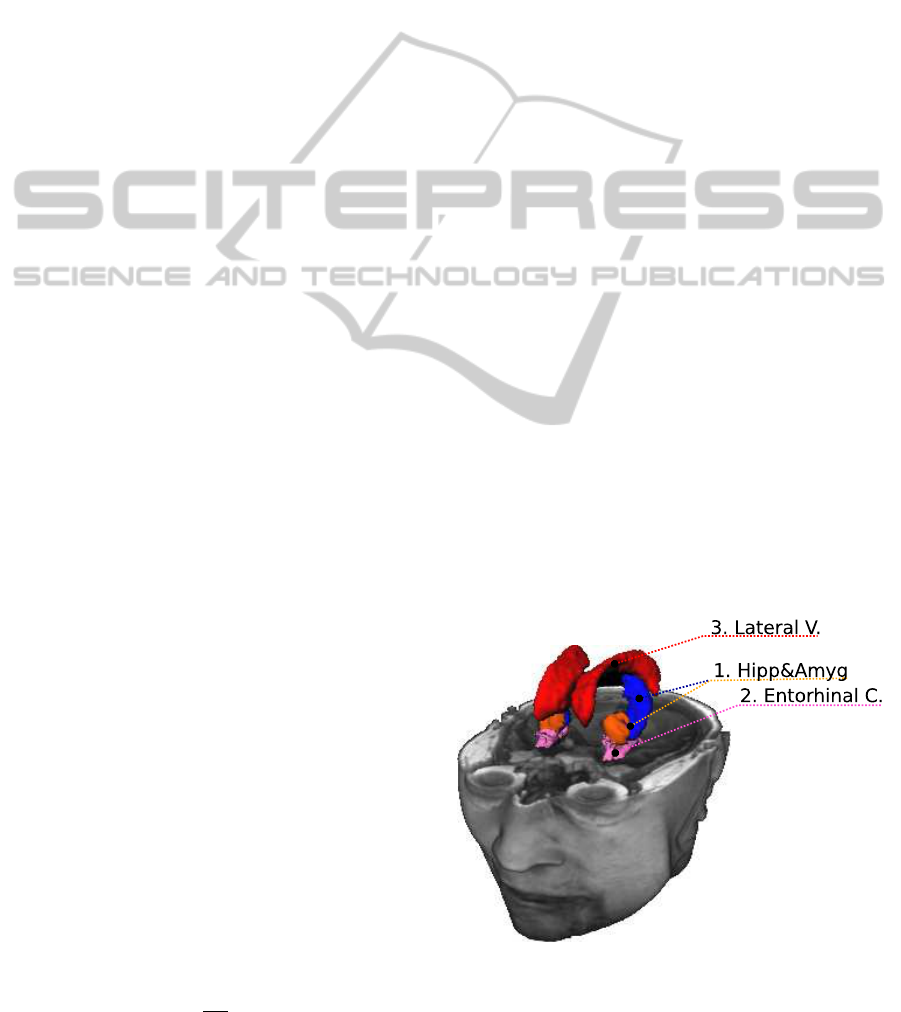
Figure 1: Analyzed brain sub-networks.
gional volumetric maps (so called RAVENS maps)
were created (Goldszal et al., 1998). Results of clas-
sification via leave-one-out cross validation method
were 94.3% for AD vs NC, 81.8% for MCI vs NC and
74.3% for MCI vs AD (Fan et al., 2008). (Davatzikos
et al., ) using the brain watershed-based clustering
method and other techniques described in (Goldszal
et al., 1998) tries to distinguish between the MCI
and NC subjects using only cross-sectional data. Ap-
plying leave-one-out procedure with SVM non-linear
classifier for the 30 subjects he receives accuracy of
90%.
2.2 Atlas based Approach
Atlas based segmentation is common technique par-
cel brain into non-overlapping, anatomical regions.
An unseen image is registered with labeled atlas and
labels are transposed onto the unseen subject’s vol-
ume. (Magnin et al., 2009) in his study after register-
ing brains with MNI152 template parceled them into
90 regions of interest (ROI). The white matter for 34
most significant sub-networks was selected and mod-
eled by Gaussian distribution. SVM with radial basis
function was used for classification. (Magnin et al.,
2009) claims specificity 96.6%, sensitivity 91.5%.
(Desikan et al., 2009) after atlas registration, selected
entorhinal cortex thickness, hippocampal volume and
supra-marginalgyrus thickness as disease progression
markers. Authors report specificity of 91% and sen-
sitivity of 90% for the cohort based on the ADNI
database when he tried to separate the MCI and NC
subjects, and ideal results for the AD vs NC classifi-
cation. (Kloppel et al., 2008) after performing atlas
registration, uses only the region cropped from vol-
ume around hippocampus region (12× 16× 12 mm)
to classify between the AD vs NC, which results with
sensitivity 75.8%, specificity 91.2%.
2.3 Volume of Interest Analysis
Methods of this group are closely related to the at-
las based approach. In most of cases atlas registra-
tion is used to segment the desired subnetwork from
the other brain tissues. The difference is, that in sub-
network of interest approach whole classification pro-
cedure is dependent upon the features extracted from
one region solely, rather than on network of differ-
ent regions. Moreover, the registration step is often
used only as an initialization step for more complex
algorithm. Most authors rely on subnetwork of hip-
pocampus solely. Nevertheless, according to (Braak
and Braak, 1997) there is an evidence that early AD
pathologymay start in entorhinal cortex and only then
EarlyAlzheimer'sDiseaseProgressionDetectionusingMulti-subnetworksoftheBrain
685

progress to hippocampus.
Labor intensive methods involving manual region
delineation of hippocampus and entorhinal cortex
were performed by (Pennanen et al., 2004), (Juotto-
nen et al., 1998) and (Du et al., 2001). For AD/NC
classification accuracy was in range from 86-91 % if
hippocampus was used and 82-83 % if entorhinal cor-
tex volume was as an input. In MCI/NC case accu-
racies were 60-70 % for hippocampus and 66 % for
entorhinal cortex volume. Important conclusion was
that incorporating few subnetworks together can im-
prove overall results, for example in AD case if both
sub-network volumes were incorporated accuracy im-
proved by +3 % (Du et al., 2001).
(Fan et al., 2008) in the second part of his study
used the volume of hippocampus (left and right)
against the entorhinal cortex (left and right) after nor-
malization by intra-cranial volume. The received ac-
curacy using linear-SVM and leave-one-outcross val-
idation was 82.0% for AD vs NC 76.0% for MCI/NC,
and AD/MCI 58.3% respectively. (Chupin et al.,
2009) proposed fully automatic approach based on
anatomical priors for the hippocampus region extrac-
tion. Leave-one-out approach was used for testing.
This method proved to be accurate in 76-80 % in
NC/AD classification case. (Lotjonen et al., 2011)
proposes to perform the automatic hippocampus ex-
traction based on multi-atlas segmentation frame-
work, adding the partial volume effect correction
(Tohka et al., 2004). The basic idea is to register non-
rigidly the unseen data with a template and to select
the most similar atlas compared to the registered un-
seen data. Tissue class having the highest probabil-
ity in voxel is chosen as feature for final segmenta-
tion. Simplest linear classifier was used with accuracy
75.0 % in AD/NC case.
(Gerardin et al., 2009) uses hippocampus segmen-
tation method provided by (Chupin et al., 2009) as
a first step, followed by hippocampus shape descrip-
tion by spherical harmonics coefficients. It is a math-
ematical approachto represent surfaces with spherical
topology, which can be seen as 3D Fourier series ex-
pansion (Gerardin et al., 2009). The best combination
of parameters gave sensitivity 96 % and specificity of
92 % in AD vs NC classification. MCI vs NC case
best result was sensitivity 83 %, specificity 84 %. Re-
sults were validated for only 23 AD and 23 MCI sub-
jects.
3 SUBJECTS
We studied and analyzed data of 48 patients
with AD (25 males, 23 females, age±standard-
deviation (SD)=76.6 ± 6.3, Mini Mental State Ex-
amination (MMSE)±(SD)=23.5 ± 1.9), 119 subjects
with MCI (79 males, 40 females, age±(SD)=75.1±
7.4, (MMSE)±(SD)=27.2 ± 1.6) and 66 NC sub-
jects (40 males, 26 females, age±(SD)=76.3 ±
4.6, (MMSE)±(SD)=29.2± 0.9) recruited for ADNI
study. Provided MMSE scores correspond the
first screening at the hospital. Detailed subject
list with ID for ADNI database can be found at
http://pages.cs.wisc.edu/˜hinrichs/
. All the
subjects were followed up for two years, therefore
data was collected during the first visit and the same
procedures repeated in two years.
ADNI eligibility criteria in detail are described at
http://www.adni-info.org
. Briefly the subjects
are 55-90 years old, if they havea memory complains.
Have to be fluent in Spanish or English, accompany-
ing person has to be present. Specific psychoactive
medications are excluded (Fennema-Notestine et al.,
2009). In this study all the ADNI subjects will be di-
vided into 3 groups, based on criteria as follows:
• Normal Cognitive (NC) - Mini-Mental State
Examination (MMSE) scores between 24 and
30 (maximal), CDR of 0 (3 maximal), non-
depressed, no memory complains.
• Mild Cognitive Impairment (MCI) - MMSE
scores between 24 and 30, memory complaint,
preferably corroborated by an informant, objec-
tive memory loss measured by a education ad-
justed scores on Wenchsler Memory Scale Logi-
cal Memory, a CDR of 0.5, absence of significant
levels of impairment in other cognitive domains,
essentially preserved activities of daily living.
• Alzheimer’s Disease Subject (AD) - MMSE
scores between 20 and 26, CDR 0.5 or 1, mem-
ory complaint.
4 METHODS
Volumetric measures were created in 7 subcortical re-
gions: hippocampus, amygdala, caudate, thalamus,
pallidus, putamen, and two brain ventrical networks,
namely lateral and 3rd ventricle. In addition, two gray
matter structures temporal pole and entorhinal cortex.
All together 10 different brain regions were investi-
gated. Automatic 3D whole-brain segmentation pro-
cess was based on publicly available FreeSurfer soft-
ware package.
All experiments were performed using the sta-
ble release v5.1.0 with a HP Z800 workstation (pa-
rameters: 94.6 GB of RAM memory, 64-bit Intel
R
Xeon
R
Six-Core Processor X5670 with a processing
IJCCI2012-InternationalJointConferenceonComputationalIntelligence
686
speed 2.93 GHz, 12 MB cache). During all the ex-
periments Ubuntu 11.10, 64-bit operating system was
used. The average processing time for one subject
was 12 hours. After automatic processing was fin-
ished all the subjects were checked manually for the
artifacts and segmentation errors.
Before we can measure individual volumes for
the different subcortical structures we should decide
“how to normalize brain size variability among dif-
ferent subjects?”. According to our measurements
registering all the brains with a MNI152 template
(a 9 degrees of freedom affine transformation was
used; transformation matrix was calculated using
FreeSurfer software) gave better results, than struc-
ture normalization by cortical area. By better we
mean, that differences between the subject groups in
first case were larger compared to normalization by
cortical volume, leading to better AUC scores.
We analyzed two approaches. First, each extracted
sub-network volume was used solely as an input fea-
ture. Each sub-network was described by 3 features:
• V
SN
M
00
,mm
3
– structure volume at the base line visit
(month M
00
), for the structure name SN.
• V
SN
M
24
,mm
3
– structure volume after 24 months had
passed from the base line visit, for the structure
name SN
• V
SN
∆
24
,% – structure volume change in 24 month.
This criteria was added to have one dimensionless
descriptor for the each volume.
Moreover, we proposeone new sub-network. Hip-
pocampus and amygdala are close to indistinguish-
able using only the intensity information available in
MRI (Fischl et al., 2002). Therefore, automatic soft-
ware performs the segmentation based on the spatial
information provided by the atlas and local spacial re-
lationship, such as “posterior amygdala is frequently
superior to anterior hippocampus, but never inferior
to it” (Fischl et al., 2002). Therefore, we propose to
integrate these volumes, since they are neighbors and
the border between them is hard to define. We call our
new marker HA or hippocampus+amygdala.
Each feature was checked for its suitability to be
employed for the automatic classification. This was
done by evaluating the AUC for each feature, together
with Fisher score (equation 1), due to it’s close rela-
tion with LDA. The main advantage of AUC over the
Fisher score is that it provides a non-parametric rep-
resentation of the diagnostic accuracy of the feature.
Moreover, features from completely different sources
or studies can be compared to each other by comput-
ing
F =
S
B
S
W
. (1)
Here, in a 2 class case, S
B
presents the so called be-
tween class scatter of the original feature vectors:
S
B
= µ
1
− µ
2
. (2)
µ
i
- is the mean for each class i, while S
W
presents
within class scatter:
S
W
= σ
1
2
+ σ
2
2
. (3)
where, σ
i
- is a measure of variability in each class i.
At the first stage, we performed classification us-
ing each feature separately. Then we tested a new,
multi-volume based approach. It utilizes a group of
the subnetwork based features, rather than on any sin-
gle feature. The vector was constructed by sorting
the features according their Fisher score in descend-
ing fashion, similar to:
~
V = [V
Hp
M00
,V
Hp
M24
,∆
Hp
24
,V
Am
M00
,...,∆
LastVolume
24
], (4)
where, Hp stands for the hippocampus and Am for
amygdala.
Starting with a single feature, with each subse-
quent iteration we includedextra feature as an input to
the classificator. Since we used 9 subnetworks(amyg-
dala and hippocampus were integrated) in our study
and 3 descriptors per each volume in the final itera-
tion there was 27 features used as an input data.
5 RESULTS
The best discriminative abilities have volumes of the
hippocampus (AUC = 0.86), amygdala (AUC = 0.85)
and entorhinal cortex (AUC = 0.80) in both AD and
MCI cases (fig. 2) indicating that disease mostly pro-
gresses in medial temporal lobe and it’s subnetworks.
Figure 2: The most discriminative regions in AD and MCI
cases: 1) Hippocampus and Amygdala; 2) Entorhinal Cor-
tex; 3) Lateral Ventricle (only in AD case, in MCI case sub-
stituted by pallidus).
EarlyAlzheimer'sDiseaseProgressionDetectionusingMulti-subnetworksoftheBrain
687
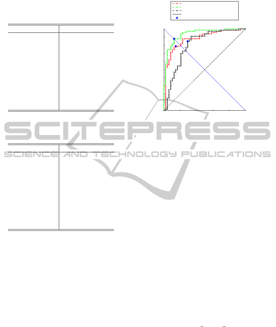
Table 1: AUC scores for investigated structures (V
M
00
and
V
M
24
are given in mm
3
, andV
∆
24
in % from V
M
00
) in AD/NC
case.
Feature Name V
M
00
V
M
24
V
∆
24
Hipp.+Amyg. 0.88 0.94 0.81
Hippocampus 0.86 0.92 0.82
Amygdala 0.85 0.91 0.70
Entorhinal Cortex 0.80 0.92 0.78
Lateral Ventricle 0.68 0.76 0.61
Putamen 0.60 0.75 0.71
Caudate 0.57 0.47 0.60
Thalamus 0.57 0.70 0.61
Temporal Pole 0.56 0.71 0.74
3rd Ventricle 0.51 0.58 0.53
Pallidus 0.50 0.62 0.61
Table 2: AUC scores for investigated structures (V
M
00
and
V
M
24
are given inmm
3
, andV
∆
24
in % fromV
M
00
) in MCI/NC
case.
Feature Name V
M
00
V
M
24
V
∆
24
Hipp.+Amyg. 0.71 0.74 0.67
Hippocampus 0.71 0.74 0.66
Amygdala 0.68 0.70 0.62
Entorhinal Cortex 0.64 0.69 0.59
Pallidus 0.62 0.59 0.51
Thalamus 0.61 0.61 0.53
Putamen 0.59 0.60 0.57
Temporal Pole 0.56 0.58 0.55
Caudate 0.55 0.52 0.53
Lateral Ventricle 0.54 0.56 0.57
3rd Ventricle 0.53 0.54 0.51
The results for the AUC scores are presented in ta-
bles 1 for AD/NC case and 2 for MCI/NC case. Also
figure 3 presents all 3 ROC curves for the AD/NC
case. In both cases the best discriminative ability had
been shown by integrated hippocampusand amygdala
volume. Therefore, for our classification task instead
of separate amygdala and hippocampus volumes, we
will use the integrated one. Second remark would
be, that the discriminative strength increases as time
passes. It’s due to fact, that in AD (same as MCI) the
subject’s brain deteriorates faster compared to a NC
subject. Thus, differences between structures become
bigger in two years. Therefore, they have more dis-
criminative power.
Finally, the last remark would be, that in both AD
and MCI cases, the cross-sectional differences V
M
00
and V
M
24
, show better AUC scores, compared to the
longitudinal changes in volume, presented by V
∆
24
.
This indicates, that incubating period for the disease is
long. Therefore, volume change in 2 years is weaker
compared to ones, happened before the subject has
0 0.2 0.4 0.6 0.8 1
0
0.1
0.2
0.3
0.4
0.5
0.6
0.7
0.8
0.9
1
False positive rate (1−Specificity)
True positive rate (Sensitivity)
ROC curve for Hippocampus+Amygdala (NC vs AD)
ROC at M00 (AUC=0.88)
ROC at M24 (AUC=0.94)
ROC for Delta24 (AUC=0.81)
Random classifier
Cut−off point
Figure 3: ROC curve in AD/NC case for the best MRI data
based feature – Hippocampus+Amygdala. V
M
00
– red line,
V
M
24
– blue line, V
∆
24
– black line.
been included to the study. The other way around, it
can happen that some NC subjects are on a way to
develop dementia, and the shrinkage of some brain
subnetworks just started recently. Therefore, while
the absolute volumes of the subnetworks are still rela-
tively large, they start to shrink with intensity compa-
rable to the MCI or AD groups, so we shouldn’t rely
on the volume changes solely.
5.1 Classification
To evaluate automatic classification results we used
Linear Discriminant Analysis (LDA) and Quadratic
Discriminant Analysis (QDA). These methods max-
imize ratio of between-class variance to the within-
class variance in any particular data set and guar-
antees maximal separability. These classificators in
contrast to Support Vector Machines (SVM) are pa-
rameter free. Therefore it is easy to interpret results.
Leave-one-outwas used as a cross-validation strategy.
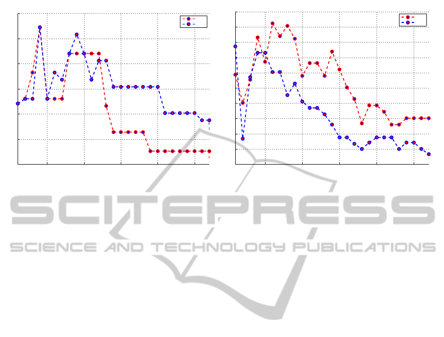
The accuracy in the figures 4(a), 4(b), 5(a) and
5(b) is presented by means of balanced Accuracy
(b − ACC) in y-axis, which represents the averaged
sensitivity and specificity value:
b− ACC =
1
2
SEN+
1
2
SPE, (5)
here, SEN - sensitivity, SPE - specificity.
Single Feature, AD vs NC. The results of cross val-
idation are presented in figure 4(a). None of the sin-
gle features is able to perform ideal classification.
The best MRI based marker performance was ob-
tained by hippocampusat M
00
with b−ACC = 84.4%,
while integrated hippocampus and amygdala volumes
IJCCI2012-InternationalJointConferenceonComputationalIntelligence
688

0.45
0.5
0.55
0.6
0.65
0.7
0.75
0.8
0.85
0.9
Structure name
b−ACC
AD vs NC for Single Feature
Hipp+Amyg
Hipp
Amyg
Entor
Pal
Thal
Put
TempP
Caud
LatV.
3Vent
M00 LDA
M00 QDA
M24 LDA
M24 QDA
D24 LDA
D24 QDA
(a)
0.4
0.45
0.5
0.55
0.6
0.65
0.7
0.75
Structure name
b−ACC
MCI vs NC for Single Feature
Hipp+Amyg
Hipp
Amyg
Entor
Pal
Thal
Put
TempP
Caud
LatV.
3Vent
M00 LDA
M00 QDA
M24 LDA
M24 QDA
D24 LDA
D24 QDA
(b)
Figure 4: Accuracy for LDA (dashed line) and QDA (dotted line) in Single-Feature case, for V
M
00
- red, V
M
24
- blue, V
∆
24
-
black lines in (a) AD/NC (b) MCI/NC cases.
were right behind, with b − ACC = 83.9% at M
00
.
But at M
24
best b − ACC belongs already to hip-
pocampus+amygdala with b − ACC = 85.4% (SEN
= 80.3%, SPE = 87.5%), while hippocampus solely
scores b − ACC = 84.4%. Generally speaking most
of MRI based features improved as time passed, ex-
cept for caudate and 3rd ventricle. While the relative
change V
∆
24
shows better results only in the case of
the temporal pole, possibly indicating that the sub-
network is involved in the disease at a later stages.
Moreover, in the most cases LDA showed better clas-
sification results than QDA.
Single Feature, MCI vs NC. The same procedure
was repeated for the MCI vs NC subjects. The
b − ACC results are summarized in the figure 4(b).
The best discriminative ability at V
M
00
is shown by
entorhinal cortex with b− ACC = 67.9%, followed by
hippocampus (66.2%) and hippocampus and amyg-
Table 3: Five best features, represented by Sensitivity and
Specificity values with LDA classifier for investigated fea-
tures in AD/NC case (HA - hippocampus+amygdala, Hp -
hippocampus, Am - amygdala, EC - entorhinal cortex, LV
- lateral venricle).
Name V
M
00
V
M
24
V
∆
24
SEN SPE SEN SPE SEN SPE
HA 80.3 87.5 83.3 87.5 84.8 68.8
Hp 83.3 85.4 83.3 85.4 84.8 66.7
Am 81.8 77.1 86.4 83.3 72.7 60.4
EC 75.8 72.9 83.3 81.2 81.8 64.6
LV 72.7 60.4 75.8 66.7 62.1 56.2
dala combined volumes (64.7%). While after two
years, the best discriminative abilities shift to hip-
pocampus+amygdala (69.7% with QDA classifica-
tor), followed by hippocampus (68.4%) and amyg-
dala (66.4%), while entorhinal cortex declines to
66.7%. Relative changes based features presented re-
sults were worse compared to the absolute volume
data, except for putamen and lateral ventricle, but in
both cases results were close to random.
Multi-feature, AD vs NC. The second approach was
to combine the strongest markers together. First we
use training set, to sort features in descending order,
according to their Fisher score. The 7 most discrimi-
native features in AD/NC were:
~
V = [V
HA
M
24
,V
Ent
M
24
,V
HA
M
00
,V
Ent
M
00
,V
Ent
∆
24
,V
HA
∆
24
,V
Lat
M
24
]. (6)
Starting from the most important feature, we in-
clude less important ones in each iteration. So, if
Table 4: Five best features represented by their Sensitivity
and Specificity values with LDA classifier for investigated
features in MCI/NC case (HA - hippocampus+amygdala,
Hp - hippocampus, Am - amygdala, EC - entorhinal cortex,
Pl - pallidus).
Name M
00
M
24
V
∆
24
SEN SPE SEN SPE SEN SPE
HA 69.7 59.7 72.7 63.0 66.7 57.1
Hp 72.7 59.7 71.2 65.5 68.2 54.6
Am 68.2 59.7 69.7 63.0 59.1 56.3
EC 72.7 63.0 65.2 68.1 60.6 47.1
Pl 60.6 60.5 57.6 56.3 43.9 48.7
EarlyAlzheimer'sDiseaseProgressionDetectionusingMulti-subnetworksoftheBrain
689
5 10 15 20 25
0.83
0.84
0.85
0.86
0.87
0.88
0.89
Nr of Features
b−ACC
AD vs NC Multi Features
LDA
QDA
(a)
5 10 15 20 25
0.62
0.63
0.64
0.65
0.66
0.67
0.68
0.69
0.7
0.71
0.72
Nr of Features
b−ACC
MCI vs NC Multi Features
LDA
QDA
(b)
Figure 5: Accuracy for LDA (red) and QDA (blue) in Multi-Feature case (a) AD/NC (b) MCI/NC cases.
in first iteration we use one feature, namely hip-
pocampus V
HA
M
24
and the result is exactly the same as
if single feature would be used. Next iteration we
add entorhinal cortex, and the feature vector becomes
[V
HA
M
24
,V
Ent
M
24
], this is continued until all the features are
included. Using 9 volumes (volumes of hippocampus
and amygdala were combined together), we have 27
features. Results for the full feature vector are pre-
sented in figure 5(a) for AD/NC case and 5(b) for
MCI/NC case.
The best obtained accuracy was, when first 3 fea-
tures were used, and is equal to b − ACC = 88.5%
(SEN=87.9%, SPE=89.1%). Results obtained by the
multi-approach are better than based on single feature
approach by 4.5%.
Multi-feature, AD vs MCI. The best accuracy was
71.2% (SEN = 72.7%, SPE = 69.8%) when 6 fea-
tures were used (LDA). 7 most discriminative features
were:
~
V = [V
HA
M
24
,V
HA
M
00
,V
EC
M
24
,V
HA
∆
24
,V
Ent
M
00
,V
Tl
M
24
,V
Tl
M
00
]. (7)
5 from the 6 strongest features in MCI case be-
long, to hippocampus, amygdala and entorhinal cor-
tex regions. This confirms one more time that disease
starts it’s progression in the sub-networks of medial
temporal lobe.
Compared with single feature case, where the best
accuracy score was from 69.7 % for V
HA
M
24
, result im-
proved by 1.5% and became 71.2%.
6 CONCLUSIONS
1. We propose the integrated marker, consisting of
hippocampus and amygdala volumes improves
the AUC for M
00
and M
24
. Proposed marker
improves ROC curve compared to hippocam-
pus or amygdala volumes separately in both AD
(AUC
M
00
= 0.88, AUC
M
24
= 0.94, AUC
∆24
=
0.81) and MCI (AUC
M
00
= 0.71, AUC
M
24
= 0.74,
AUC
∆24
= 0.67) cases.
2. The best score for a single feature was obtained
when hippocampus+amygdala marker was used
with b − ACC = 85.4% (SEN = 80.3%, SPE =
87.5%) in AD and 67.9% (SEN = 72.7%, SPE =
63.0%) in MCI case.
3. Multi-Feature approach gives the classification re-
sults improvement by 4.5% compared to the sin-
gle feature case for AD/NC classification. The
best result was 88.5% (SEN = 87.9%, SPE =
89.1%) when 3 features were used. In MCI case
using our approach we improved accuracy by
1.5% and is equal to b − ACC = 71.2% (SEN=
72.7%, SPE = 69.8%) when 6 features were used.
In both AD/NC and MCI/NC cases QDA didn’t
show any significant advantage over LDA.
REFERENCES
Braak, H. and Braak, E. (1997). Staging of alzheimer-
related cortical destruction. Int Psychogeriatry, 9
Suppl 1.
Chupin, M., Gerardin, E., Cuingnet, R., Boutet, C.,
Lemieux, L., Lehericy, S., Benali, H., Garnero, L.,
and Colliot, O. (2009). Fully automatic hippocampus
segmentation and classification in alzheimer’s disease
and mild cognitive impairment applied on data from
adni. Hippocampus, 19(6):579–587.
Davatzikos, C., Fan, Y., Wu, X., Shen, D., and Resnick,
S. M. Detection of prodromal alzheimer’s disease via
IJCCI2012-InternationalJointConferenceonComputationalIntelligence
690

pattern classification of magnetic resonance imaging.
Neurobiology of Aging, 29(4):514–523.
Desikan, R. S., Cabral, H. J., Hess, C. P., Dillon, W. P.,
Glastonbury, C. M., Weiner, M. W., Schmansky, N. J.,
Greve, D. N., Salat, D. H., Buckner, R. L., Fischl, B.,
and Initiative, A. D. N. (2009). Automated mri mea-
sures identify individuals with mild cognitive impair-
ment and alzheimer’s disease. Brain, 132(8):2048–
2057.
Du, A. T., Schuff, N., Amend, D., Laakso, M. P., Hsu,
Y. Y., Jagust, W. J., Yaffe, K., Kramer, J. H., Reed, B.,
Norman, D., Chui, H. C., and Weiner, M. W. (2001).
Magnetic resonance imaging of the entorhinal cortex
and hippocampus in mild cognitive impairment and
alzheimer’s disease. Journal of Neurology, Neuro-
surgery & Psychiatry, 71(4):441–447.
Fan, Y., Batmanghelich, N., Clark, C. M., and Davatzikos,
C. (2008). Spatial patterns of brain atrophy in mci
patients, identified via high-dimensional pattern clas-
sification, predict subsequent cognitive decline. Neu-
roImage, 39(4):1731–1743.
Fennema-Notestine, C., Hagler, D. J., McEvoy, L. K.,
Fleisher, A. S., Wu, E. H., Karow, D. S., and Dale,
A. M. (2009). Structural mri biomarkers for preclini-
cal and mild alzheimer’s disease. Human Brain Map-
ping, 30(10):3238–3253.
Fischl, B., Salat, D. H., Busa, E., Albert, M., Dieterich,
M., Haselgrove, C., van der Kouwe, A., Killiany, R.,
Kennedy, D., Klaveness, S., Montillo, A., Makris, N.,
Rosen, B., and Dale, A. M. (2002). Whole brain
segmentation: Automated labeling of neuroanatomi-
cal structures in the human brain. Neuron, 33(3):341–
355.
Gerardin, E., Chetelat, G., Chupin, M., Cuingnet, R., Des-
granges, B., Kim, H.-S., Niethammer, M., Dubois, B.,
Lehericy, S., Garnero, L., Eustache, F., and Colliot, O.
(2009). Multidimensional classification of hippocam-
pal shape features discriminates alzheimer’s disease
and mild cognitive impairment from normal aging.
NeuroImage, 47(4):1476–1486.
Goldszal, A. F., Davatzikos, C., Pham, D. L., Yan, M. X.,
Bryan, R. N., and Resnick, S. M. (1998). An image-
processing system for qualitative and quantitative vol-
umetric analysis of brain images. Journal Of Com-
puter Assisted Tomography, 22(5):827–837.
Juottonen, K., Laakso, M., Insausti, R., Lehtovirta, M.,
Pitknen, A., Partanen, K., and Soininen, H. (1998).
Volumes of the entorhinal and perirhinal cortices in
alzheimers disease. Neurobiology of Aging, 19(1):15–
22.
Kloppel, S., Stonnington, C. M., Chu, C., Draganski, B.,
Scahill, R. I., Rohrer, J. D., Fox, N. C., Jack, C. R.,
Ashburner, J., and Frackowiak, R. S. J. (2008). Auto-
matic classification of mr scans in alzheimer’s disease.
Brain, 131(3):681–689.
Lotjonen, J., Wolz, R., Koikkalainen, J., Julkunen, V., Thur-
fjell, L., Lundqvist, R., Waldemar, G., Soininen, H.,
and Rueckert, D. (2011). Fast and robust extraction
of hippocampus from mr images for diagnostics of
alzheimer’s disease. NeuroImage, 56(1):185–196.
Magnin, B., Mesrob, L., Kinkingnhun, S., Plgrini-Issac,
M., Colliot, O., Sarazin, M., Dubois, B., Lehricy, S.,
and Benali, H. (2009). Support vector machine-based
classification of alzheimers disease from whole-brain
anatomical mri. Neuroradiology, 51:73–83.
Pennanen, C., Kivipelto, M., Tuomainen, S., Hartikainen,
P., Hnninen, T., Laakso, M. P., Hallikainen, M., Van-
hanen, M., Nissinen, A., Helkala, E.-L., Vainio, P.,
Vanninen, R., Partanen, K., and Soininen, H. (2004).
Hippocampus and entorhinal cortex in mild cogni-
tive impairment and early ad. Neurobiology of Aging,
25(3):303–310.
Tohka, J., Zijdenbos, A., and Evans, A. (2004). Fast and ro-
bust parameter estimation for statistical partial volume
models in brain mri. NeuroImage, 23(1):84–97.
Vemuri, P., Gunter, J. L., Senjem, M. L., Whitwell, J. L.,
Kantarci, K., Knopman, D. S., Boeve, B. F., Petersen,
R. C., and Jr., C. R. J. (2008). Alzheimer’s disease di-
agnosis in individual subjects using structural mr im-
ages: Validation studies. NeuroImage, 39(3):1186–
1197.
EarlyAlzheimer'sDiseaseProgressionDetectionusingMulti-subnetworksoftheBrain
691
