BSAR SIGNAL MODELING AND SLC IMAGE
RECONSTRUCTION
T.P. Kostadinov, A.D. Lazarov
Institute of Information and Communication Technologies, Bulgarian Academy of Sciences, G. Bonchev 2, Sofia, Bulgaria,
Dept. of Informatics and Technical Sciences Burgas Free University, San Stefano 63 Burgas, Bulgaria
Keywords: BSAR, SLC, signal model, kinematics.
Abstract: In this paper, a Bistatic Synthetic Aperture Radar (BSAR) signal model and Single Look Complex (SLC)
image obtained by multiple satellite BSAR system are considered. Geometry and kinematics of BSAR
scenario, including a BSAR satellite transmitter and multiple receivers as well as a complicated surface of
observation are described. BSAR signal model based on linear frequency modulated emitted waveform and
BSAR scenario is derived. Standard Fourier transformation is applied to extract an SLC BSAR image of
high quality on range and cross range directions. To verify the BSAR signal model and image extraction
procedure a numerical experiment is carried out.
1 INTRODUCTION
In recent years raise in the interest of Bistatic
Synthetic Aperture Radar (BSAR) technology is a
fact. BSAR concept in SAR for Earth observation
and BSAR spaceborne performance are analyzed in
(
Moccia A., 2002). Application of a BSAR method
increases the quality of imaging and improves the
functionality of the imaging radars (
Moccia, A.,
2005). Bistatic configurations of synthetic aperture
radar imaging systems have been investigated in
(Loffeld, O., 2003). New bistatic SAR techniques
for imaging are proposed in (Ender, J. H. G, 2004).
The problems of the focusing of SAR image are
considered in (D’Aria, D., 2004). Passive space-
surface bistatic SAR for local area monitoring is
described in (Cherniakov M., 2009). Maritime target
cross section estimation for an ultra-wideband
forward scatter radar network is considered in
(Daniel L., 2008). Results of a space-surface bistatic
SAR image formation algorithm are presented in
(Antoniou M., 2007).
BSAR in essence is a bistatic configuration, with a
moving satellite transmitter, and two or more
stationary receivers, spatially separated by a base
line. The scene of observation includes stationary
and/or moving objects. In latter case the system is
referred to Generalized Bistatic Inverse Synthetic
Aperture Radar (BISAR).
In the present work a scenario with satellite
transmitter two receivers and stationary object is
discussed. All components of bistatic SAR
configuration are described in one and the same
coordinate system. First, an accent is made on
definition and implementation of BSAR geometry
and kinematical vector equations. Second, a special
attention is dedicated to processes of BSAR signal
formation and image reconstruction procedure that
comprises range and azimuth compressions
implemented by Fourier transforms.
The rest of the paper is organized as follows. In
Section 2 BSAR scenario that comprises geometry
and kinematical equations of satellite transmitter
carrier is described. In Section 4 a linear frequency
waveform and BSAR signal model in topology with
one satellite transmitter and two receivers are
discussed in details. In Section 4 an image
reconstruction algorithm is derived. In Section 5
results of a numerical experiment are graphically
illustrated and thoroughly discussed. In Section 6
conclusions are made.
65
Kostadinov T. and Lazarov A.
BSAR SIGNAL MODELING AND SLC IMAGE RECONSTRUCTION.
DOI: 10.5220/0005414000650071
In Proceedings of the First International Conference on Telecommunications and Remote Sensing (ICTRS 2012), pages 65-71
ISBN: 978-989-8565-28-0
Copyright
c
 2012 by SCITEPRESS – Science and Technology Publications, Lda. All rights reserved

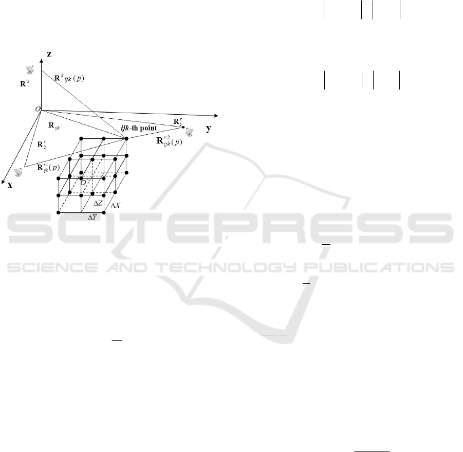
2 BSAR GEOMETRY
Three dimensional (3-D) BSAR scenario presented
in Fig. 1 comprises satellite transmitter described by
current position vector in discrete time
instant p, stationary receivers described by current
position vectors and , and a target of
interest, all situated in Cartesian coordinate system
Oxyz. The target is presented as an assembly of point
scatterers in the same Cartesian coordinate system as
the transmitter and the receivers.
)(p
s
R
r
1
R
r
2
R
Figure 1: 3-D geometry of BSAR scenario
Denote as a
range distance vector measured from the satellite
transmitter with the current vector position to
the ijkth point scatterer of the object space at the
moment p, is described by the vector equation
[]
T
ijkijkijk
ijk
s
pzpypxp )(),(),()( =R
)(p
s
R
ijkp
s
ijk
s
Tp
N
pp RVRR +
⎟
⎠
⎞
⎜
⎝
⎛
−+=
2
)()(
(1)
where V is the satellite’s vector-velocity, is the
pulse repetition period, N is the number of emitted
pulses
p
T
T
ijkijkijkijk
zyx ],,[=R
(2)
is the position vector of the target.
Range distance vector between the ijkth point
scatterer and the first receiver is defined by:
ijk
r
ijk
r
RRR −=
1
1
(3)
Range distance vector between ijkth point scatterer
and the second receiver is defined by:
ijk
r
ijk
r
RRR −=
2
2
(4)
Round trip distance transmitter-ijkth point scatterer-
first receiver expressed as
ijk
r
ijk
s
ijk
ppR
11
)()( RR +=
.
(5)
Round trip distance transmitter-ijkth point scatterer-
second receiver expressed as
ijk
r
ijk
s
ijk
ppR
12
)()( RR +=
.
(6)
3 LFM PULSES AND BSAR
SIGNAL MODEL
The satellite transmitter transmits a series of
electromagnetic waves to the moving target, which
are described analytically by sequence of N linear
frequency modulated pulses each of which is
described by
[]
{
}
2
)( bttj
T
t
tS +ω−= exprect
&
,
(7)
where
λ
π=ω
c
2
is the angular frequency;
=
c
8
10.3
m/s is the speed of the light; λ is the wavelength of
the signal; T is the time duration of a LFM pulse;
T
F
b
Δ
π
=
2
is the LFM rate. The bandwidth of the
transmitted pulse provides the dimension of the
range resolution cell.
The deterministic component of the BSAR signal,
reflected by ijkth point scatterer of the target and
registered by first and second receiver can be
described by the expression (Lazarov A., 2011)
()
()
⎪
⎭
⎪
⎬
⎫
⎪
⎩
⎪
⎨
⎧
⎥
⎥
⎥
⎦
⎤
⎢
⎢
⎢
⎣
⎡
−+
+−ω
−×
×
−
=
2
2,1
2,1
2,1
2,1
)(
)(
)(
),(
pttb
ptt
j
T
ptt
atpS
ijk
ijk
ijk
ijk
ijk
exp
rect
&
(8)
where
First International Conference on Telecommunications and Remote Sensing
66

⎪
⎪
⎪
⎪
⎩
⎪
⎪
⎪
⎪
⎨
⎧
≥
−
<
−
<
−
≤
=
−
1
)(
,0
0
)(
,0
,1
)(
0,1
)(
2,1
2,1
2,1
2,1
T
ptt
T
ptt
T
ptt
T
ptt
ijk
ijk
ijk
ijk
rect
(9)
where is the reflection coefficient of the ijkth
point scatterer, a 3-D image function;
ijk
a
c
pR
pt
ijk
ijk
)(
)(
2,1
2,1
=
is the time delay of the signal
from the ijkth point scatterer; t is the time dwell or
the fast time of the BSAR signal which in discrete
form can be written as
Tkpkt
ijk
Δ−+= ]1)([
min
2,1
(10)
where
Kpkpkk
ijk
i
ijk
+−= )]()([,1
min
2,1
max
2,1
is the
sample number of a LFM pulse;
T
T
K
Δ
=
is the full
number of samples of the LFM pulse,
T
Δ
is the
time duration of a LFM sample,
⎥
⎥
⎥
⎥
⎤
⎢
⎢
⎢
⎢
⎡
Δ
=
T
pt
pk
ijk
ijk
)(
)(
min
2,1
min
2,1
is the number of the
radar range bin where the signal, reflected by the
nearest point scatterer of the target is detected,
c
pR
pt
ijk
ijk
)(
)(
min
2,1
min
2,1
= is the minimal time delay
of the BSAR signal reflected from the nearest point
scatterer of the target
is the relative time
dimension of the target;
)()()(
min
2,1
max
2,1
pkpkpK
ijkijk
−=
⎥
⎥
⎥
⎥
⎤
⎢
⎢
⎢
⎢
⎡
Δ
=
T
pt
pk
ijk
ijk
)(
)(
max
2,1
max
2,1
is the number of the
radar range bin where the signal, reflected by
farthest point scatterer of the target is detected;
c
pR
pt
ijk
ijk
)(
)(
max
2,1
max
2,1
= is the maximum round
trip time delay of the BSAR signal reflected from
the farthest point scatterer of the target and received
in both receivers.
The range vector coordinates from the satellite
transmitter to the ijk-th point scatterer can be
calculated by the following equations
[
]
ijkpxs
ijk
s
xpNTVxpx −−−= )2/()(
,
[
]
ijkpys
ijk
s
ypNTVypy −−−= )2/()(
,
[
]
ijkpzs
ijk
s
zpNTVzpz −−−= )2/()(
0
(11)
The distance from satellite transmitter to the ijkth
point scatterer is defined by
()()()
2
1
222
)()()()(
⎥
⎦
⎤
⎢
⎣
⎡
++= pzpypxpR
s
ijk
s
ijk
s
ijk
s
ijk
(12)
The range vector - coordinates from the ijk-th point
scatterer to the receivers can be calculated by the
following equations
ijkr
ijk
xxx −=
2,12,1
,
ijkr
ijk
yyy −=
2,12,1
,
ijkr
ijk
zzz −=
2,12,1
(13)
The distance from ijkth point scatterer to the
receivers is defined by
()()()
2
1
2
2,1
2
2,1
2
2,12,1
⎥
⎦
⎤
⎢
⎣
⎡
++=
ijkijkijkijk
zyxR
(14)
The deterministic components of the BSAR signal
return from the target and registered in first and
second receivers are defined as a superposition of
signals reflected by point scatterers placed on the
target, i.e.
()
()
∑
⎟
⎟
⎟
⎟
⎟
⎟
⎟
⎠
⎞
⎜
⎜
⎜
⎜
⎜
⎜
⎜
⎝
⎛
⎪
⎭
⎪
⎬
⎫
⎪
⎩
⎪
⎨
⎧
⎥
⎥
⎥
⎦
⎤
⎢
⎢
⎢
⎣
⎡
−+
+−ω
−×
×
−
=
∑
=
ijk
ijk
ijk
ijk
ijk
ijk
ijk
pttb
ptt
j
T
ptt
a
tpStpS
2
2,1
2,1
2,1
2,12,1
)(
)(
)(
),(),(
exp
rect
&&
(15)
BSAR Signal Modeling And SLC Image Reconstruction
67

which in discrete form can be written as
(
)
(
)
⎪
⎭
⎪
⎬
⎫
⎪
⎩
⎪
⎨
⎧
⎥
⎥
⎥
⎦
⎤
⎢
⎢
⎢
⎣
⎡
−Δ++
+−Δ+ω
−×
∑
−Δ+
=
∑
=
2
2,1
min
2,1
2,1
min
2,1
2,1
min
2,1
2,12,1
)()))((
)()))((
)())((
),(),(
ptTkpkb
ptTkpk
j
T
ptTkpk
a
tpStpS
ijkijk
ijkijk
ijk
ijkijk
ijk
ijk
ijk
exp
rect
&&
(16)
where
⎪
⎪
⎪
⎪
⎪
⎩
⎪
⎪
⎪
⎪
⎪
⎨
⎧
≥
−Δ+
<
−Δ+
<
−Δ+
≤
=
−Δ+
1
)())((
if 0
0
)())((
if 0
1
)())((
0if1
)())((
2,1
min
2,1
2,1
min
2,1
2,1
min
2,1
2,1
min
2,1
T
ptTkpk
T
ptTkpk
T
ptTkpk
T
ptTkpk
ijkijk
ijkijk
ijkijk
ijkijk
rect
(17)
where
1)]()([,0
min
2,1
max
2,1
−+−= Kpkpkk
ijkijk
.
For programming implementation all terms,
including image function , rectangular function
ijk
a
T
ptTkpk
ijkijk
)())((
2,1
min
2,1
−Δ+
rect
(18)
and exponential function
(
)
(
)
⎪
⎭
⎪
⎬
⎫
⎪
⎩
⎪
⎨
⎧
⎥
⎥
⎥
⎦
⎤
⎢
⎢
⎢
⎣
⎡
−Δ++
+−Δ+ω
−
2
2,1
min
2,1
2,1
min
2,1
)()))((
)()))((
ptTkpkb
ptTkpk
j
ijkijk
ijkijk
exp
(19)
are presented as multidimensional matrices to which
entry-wise product is applied.
Demodulation (dechirping) of the BSAR signal
return is performed by multiplication with a complex
conjugated emitted waveform, i.e.
[]
()
()
[]
2
2
2,1
2,1
2,1
22,1
(exp.
)(.
)(
exp
)(
(exp),(),(
ˆ
bttj
pttb
ptt
j
T
ptt
a
bttj
T
t
ptSptS
ijk
ijk
ijk
ijk
ijk
+ω−
⎪
⎭
⎪
⎬
⎫
⎪
⎩
⎪
⎨
⎧
⎥
⎥
⎥
⎦
⎤
⎢
⎢
⎢
⎣
⎡
−+
+−ω
×
∑
−
=
+ω−×=
rect
rect
(20)
which yields
() ()
⎭
⎬
⎫
⎩
⎨
⎧
⎥
⎦
⎤
⎢
⎣
⎡
−+ω−×
∑
−
=
)()(2exp
)(
),(
ˆ
2
2,12,1
2,1
2,1
ptbptbtj
T
ptt
aptS
ijkijk
ijk
ijk
ijk
rect
(21)
Denote the current angular frequency of emitted
LFM pulse as
btt 2)(
+
ω
=
ω
, where is the carrier
angular frequency, and b is the chirp rate,
ω
Tkt
Δ
= is
the discrete time parameter, where k is the sample
number,
T
Δ
is the sample time duration. Then the
current discrete frequency can be written as
)(2 Tkb
k
Δ
+
ω
=
ω
or
kk
kTb
k
k ωΔ=
⎟
⎠
⎞
⎜
⎝
⎛
Δ+
ω
=ω )(2
.
Then expression (24) can be rewritten as (Lazarov
A., 2011)
⎥
⎥
⎥
⎦
⎤
⎢
⎢
⎢
⎣
⎡
⎟
⎟
⎟
⎠
⎞
⎜
⎜
⎜
⎝
⎛
⎟
⎟
⎟
⎠
⎞
⎜
⎜
⎜
⎝
⎛
−ω−×
∑
−
=
2
2,12,1
2,1
2,1
)(2)(
)(2exp
)(
),(
ˆ
c
pR
b
c
pR
tj
T
ptt
aptS
ijkijk
ijk
ijk
ijk
rect
(22)
which in discrete form can be written as
⎥
⎥
⎥
⎦
⎤
⎢
⎢
⎢
⎣
⎡
⎟
⎟
⎟
⎟
⎠
⎞
⎜
⎜
⎜
⎜
⎝
⎛
⎟
⎟
⎟
⎠
⎞
⎜
⎜
⎜
⎝
⎛
−ω−×
∑
−Δ+
=
2
2,12,1
2,1
min
2,1
2,1
)(2)(
2exp
)())((
),(
ˆ
c
pR
b
c
pR
j
T
ptTkpk
apkS
ijkijk
k
ijk
ijkijk
ijk
rect
(23)
The expression (23) can be interpreted as a
projection of the three-dimensional image function
onto two-dimensional BSAR signal plane
ijk
a
First International Conference on Telecommunications and Remote Sensing
68

),(
ˆ
2,1
pkS by the projective operator, the
exponential term
⎥
⎥
⎥
⎦
⎤
⎢
⎢
⎢
⎣
⎡
⎟
⎟
⎟
⎠
⎞
⎜
⎜
⎜
⎝
⎛
⎟
⎟
⎟
⎠
⎞
⎜
⎜
⎜
⎝
⎛
−ω−
2
2,12,1
)(2)(
2exp
c
pR
b
c
pR
j
ijkijk
k
(24)
Then the 2-D mage function, can be extracted
from 2-D BSAR signal in two receivers by the
inverse operation
2,1
ijk
a
∑∑
⎥
⎥
⎥
⎥
⎥
⎥
⎥
⎦
⎤
⎢
⎢
⎢
⎢
⎢
⎢
⎢
⎣
⎡
⎟
⎟
⎟
⎟
⎟
⎟
⎟
⎠
⎞
⎜
⎜
⎜
⎜
⎜
⎜
⎜
⎝
⎛
⎟
⎟
⎟
⎠
⎞
⎜
⎜
⎜
⎝
⎛
−
−ω
=
==
N
p
K
k
ijk
ijk
k
ijk
c
pR
b
c
pR
jpkSa
11
2
2,1
2,1
2,12,1
)(2
)(
2
exp).,(
ˆ
(25)
where k is the discrete coordinate measured onto the
line of sight of the object’s geometric centre, p is
the azimuth discrete coordinate.
4 IMAGE RECONSTRUCTION
ALGORITHM
First order Taylor expansion of the exponential term
⎥
⎥
⎥
⎦
⎤
⎢
⎢
⎢
⎣
⎡
⎟
⎟
⎟
⎠
⎞
⎜
⎜
⎜
⎝
⎛
⎟
⎟
⎟
⎠
⎞
⎜
⎜
⎜
⎝
⎛
−ω
2
2,12,1
)(2)(
2exp
c
pR
b
c
pR
j
ijkijk
k
(26)
and its substitution in (23) yields the following
image extraction procedure
.
ˆ
2exp.
ˆ
2exp.
).,(
ˆ
)
ˆ
,
ˆ
(
11
2,1
2,1
⎟
⎠
⎞
⎜
⎝
⎛
π
∑
⎥
⎥
⎥
⎥
⎦
⎤
⎢
⎢
⎢
⎢
⎣
⎡
∑
⎟
⎟
⎟
⎟
⎠
⎞
⎜
⎜
⎜
⎜
⎝
⎛
⎟
⎟
⎠
⎞
⎜
⎜
⎝
⎛
π
=
==
N
pp
j
K
kk
j
kpS
kpa
N
p
K
k
ijk
(27)
Range compression
∑
⎟
⎟
⎠
⎞
⎜
⎜
⎝
⎛
π=
=
K
k
K
kk
jkpS
K
kpS
1
2,12,1
ˆ
2exp).,(
1
)
ˆ
,(
~
)
(28)
Azimuth compression
∑
⎟
⎠
⎞
⎜
⎝
⎛
π=
=
N
p
ijk
N
pp
jkpS
N
kpa
1
2,12,1
ˆ
2exp).
ˆ
,(
~
1
)
ˆ
,
ˆ
(
(29)
where
Np ,1
ˆ
=
and Kk ,1
ˆ
= are ijkth point
scatterer’s azimuth and range discrete coordinates,
respectively.
Range and azimuth (cross range) compressions are
implemented by standard fast Fourier transforms.
5 NUMERICAL EXPERIMENT
To prove the properties of the 3-D SAR signal
model with linear frequency modulation and to
verify the correctness of the BSAR image
reconstruction procedures including 2-D FFT range
compression and azimuth compression a numerical
experiment is carried out. It is assumed that the
geometry of the target and the movement of the
radar system are depicted in a 3-D Cartesian
coordinate system of observation
Oxyz
. Vector
coordinates of the initial point scatterer are as follow
m, m, m; The target object
of interest is a six storage building and has the
following dimensions – height 15m, width 120m,
dept 55 m; The satellite initial coordinates are:
0
0
=
ijk
x 0
0
=
ijk
y 0
0
=
ijk
z
5,8
−
=
s
x km, 2,1
=
s
y km, km; the
satellite velocities are m/s
200
0
=
s
z
1404==
yx
VV
0
=
z
V m/s, vector-coordinates of the firs receiver
are: km, km, m; vector-
coordinates of the second receiver are: km,
km, m. The distance between the
first receiver and the second one is a 1000 m on y
direction. This distance is called base line. The
BSAR pulse parameters: the wavelength is
m; the time duration of the LFM pulse
s; the pulse repetition period s;
the carrier frequency
5,2
1
=
r
x 2,1
1
=
r
y 300
1
=
r
z
5,2
2
=
r
x
2,2
2
=
r
y 300
2
=
r
z
2
10.3
−
=λ
6
10
−
=T
3
10.5
−
=
p
T
10
=
f GHz; the frequency
bandwidth of the LFM pulse Hz; the
number of emitted pulses N = 512, the number of
samples of LFM pulse K = 256. The mathematical
expectation of the normalized intensities of the point
scatterers placed on the ship target is .
8
10.3=ΔF
01.0=
ijk
a
BSAR Signal Modeling And SLC Image Reconstruction
69

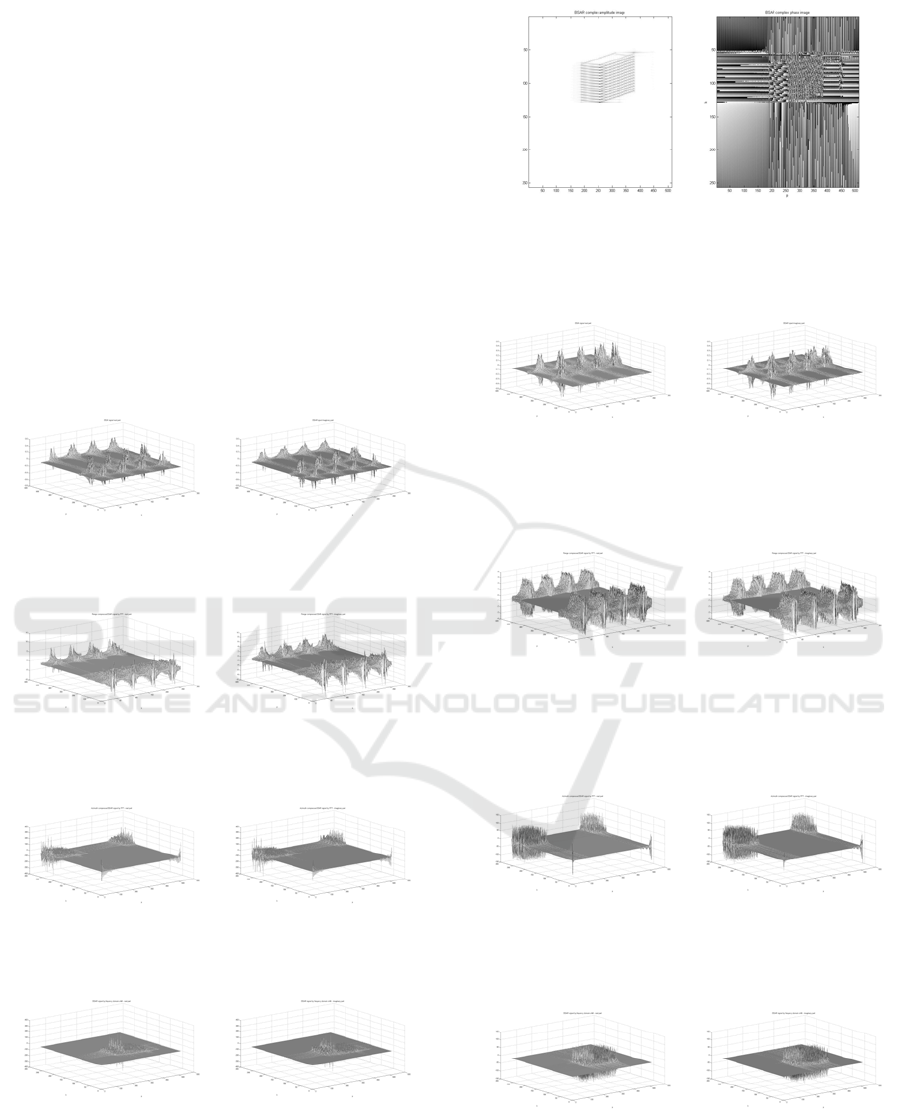
Experimental results are presented in the following
figures. In Figs. 2 and 7 a demodulated BSAR signal
with real and imaginary parts, measured in first and
second receiver, respectively, are depicted. In Figs. 3
and 8 range compressed BSAR signal with real and
imaginary parts, measured in first and second
receiver, respectively, are depicted. In Figs. 4 and 9
azimuth compressed BSAR signal with real and
imaginary parts, measured in first and second
receiver, respectively, are depicted. In Figs. 5 and 10
frequency azimuth compressed BSAR signal with
real and imaginary parts, measured in first and
second receiver, respectively, are depicted. In Figs. 6
and 11 single look complex images are presented
with a module (a) and phase (b) of the images
obtained in first and second receiver, respectively.
(a) (b)
Figure 2: Demodulated BSAR signal: real part (a),
imaginary part (b) in first receiver.
(a) (b)
Figure 3: Range compressed BSAR signal: real part (a),
imaginary part (b) in first receiver.
(a) (b)
Figure 4: Azimut compressed BSAR signal: real part(a),
imaginary part (b).
(a) (b)
Figure 5: Frequency shifted azimut compressed BSAR
signal: real part (a), imaginary part (b).
(a) (b)
Figure 6: Single looks complex image in the first receiver:
module (a), phase (b).
(a) (b)
Figure 7: Demodulated BSAR signal: real part (a),
imaginary part (b) in second receiver.
(a) (b)
Figure 8: Range compressed BSAR signal: real part (a),
imaginary part (b) in second receiver.
(a) (b)
Figure 9: Azimuth compressed BSAR signal: real part (a),
imaginary part (b) in second receiver.
(a) (b)
Figure 10: Frequency shifted azimuth compressed focused
BSAR signal: real part (a), imaginary part (b).
First International Conference on Telecommunications and Remote Sensing
70

(a) (b)
Figure 11: Single looks complex image in the second
receiver: module (a), phase (b).
The comparison analysis of two single look complex
images illustrates the functionality of the geometry,
kinematics and signal models in BSAR scenario
with multiple receivers. Between the two SLC
images there are differences in the module and phase
due to the baseline between the receivers. The phase
difference in SLC images can be used to generate a
complex interferogram that can be applied for three
dimensional measurements of the observed object.
6 CONCLUSION
In the present work BSAR approach of signal
formation and image reconstruction has been used.
Mathematical expressions to determine the range
distance to a particular point scatterer from the
object space have been derived. The model of the
BSAR signal return based on a linear frequency
modulated transmitted signal, 3-D geometry and
reflectivity properties of point scatterers from the
object space has been described. The mathematical
expression of BSAR target image – six storage
building has been derived. Based on the concept of
BSAR signal formation a classical image
reconstruction procedure including range
compression and azimuth compression implemented
by Fourier transformation has been analytically
derived. To verify the three dimensional BSAR
geometry and kinematics, signal model, algorithms
and image reconstruction, a numerical experiment
has been carried out and results have been
graphically illustrated. The multiple receiver BSAR
geometry and kinematics, equations of LFM BSAR
signal model can be used for modelling of signal
formation process and to test image reconstruction
procedures.
ACKNOWLEDGEMENTS
This work is supported by Project NATO
ESP.EAP.CLG. 983876 and Project DDVU
02/50/2010.
REFERENCES
Moccia A., Rufmo, G., D'Errico, M., Alberti G., et. al.
2002. BISSAT: A bistatic SAR for Earth observation,
In International Geoscience and Remote Sensing
Symposium (IGARSS'02), Vol. 5, June 24-28, 2002,
pp. 2628-2630.
Moccia, A., Salzillo, G., D'Errico, M., Rufino, G., Alberti,
G. 2005. Performace of bistatic synthetic aperture
radar. In IEEE Trans. on AES, vol. 41, No. 4 2005, pp.
1383 – 1395
Loffeld, O., Nies, H., Peters, V., and Knedlik, S.
2003.Models and useful relations for bistatic SAR
processing”, In International Geoscience and Remote
Sensing Symposium (IGARSS), vol. 3, Toulouse,
France, July 21—25, pp. 1442—1445.
Ender, J. H. G., Walterscheid, I., and Brenner, A. R. 2004.
New aspects of bistatic SAR: Processing and
experiments.” In International Geoscience and
Remote Sensing Symposium (IGARSS), vol. 3,
Anchorage, AK, Sept. 20—24, pp. 1758—1762.
D’Aria, D., Guarnieri, A. M., and Rocca, F. 2004.
Focusing bistatic synthetic aperture radar using dip
move out. IEEE Transactions on Geoscience and
Remote Sensing, 42, no. 7, pp. 1362—1376.
Lazarov A., Kabakchiev Ch., Rohling H., Kostadinov T.
2011. Bistatic Generalized ISAR Concept with GPS
Waveform. In 2011 IRS - Leipzig, pp. 849-854.
Lazarov A., Kabakchiev Ch., Cherniakov M., Gashinova
M., Kostadinov T. 2011. Ultra Wideband Bistatic
Forward Scattering Inverse Synthetic Aperture Radar
Imaging. In 2011 IRS - Leipzig, pp. 91-96.
Cherniakov M., Plakidis E., Antoniou M., Zuo R. 2009.
Passive Space-Surface Bistatic SAR for Local Area,
Monitoring: Primary Feasibility Study, In 2009 EuMA,
30 September - 2 October 2009, Rome, Italy
Daniel L., Gashinova M., Cherniakov M.. 2008. Maritime
Target Cross Section Estimation for an Ultra-
Wideband Forward Scatter Radar Network. In 2008
EuMA, Amsterdam, pp. 316-319.
Antoniou M., Saini R., Cherniakov M. 2007. Results of a
Space-Surface bistatic SAR image formation
algorithm, In IEEE Trans. GRS, vol. 45, no. 11, pp.
3359-3371.
BSAR Signal Modeling And SLC Image Reconstruction
71