A NEW MODEL OF THE INTERNATIONAL REFERENCE
IONOSPHERE IRI FOR TELECOMMUNICATION AND
NAVIGATION SYSTEMS
Olga Maltseva, Natalia Mozhaeva, Gennadyi Zhbankov
Institute of Physics Southern Federal University, Stachki, 194, Rostov-on-Don, Russia
Keywords: GPS. Total electron content. Ionospheric model. Radio wave propagation. Geomagnetic disturbances.
Abstract: Telecommunication, navigation, positioning systems require knowledge of ionospheric Ne(h)-profiles up to
high-altitude orbits of satellites. The only way to construct such profiles is associated with the use of the
ionospheric total electron content TEC. New option IRI-Plas of the IRI2010 model allows us to construct
Ne(h)-profiles by adjustment of the model to the current maximum values of the parameters of the
ionospheric F2 layer (foF2, hmF2) and the TEC. This paper contains a comprehensive comparison of these
profiles with the data of various experiments (ISR, CHAMP, DMSP). Results show the high efficiency of
this adjustment. The proposed method of further adjustment of the IRI-Plas model to the plasma frequency
at altitudes of CHAMP and DMSP satellites allows us to produce behaviors of Ne(h)-profiles during the
disturbances, as well as to refine the values of TEC, which determine the accuracy of positioning.
1 INTRODUCTION
The operation of the various satellite
communication, navigation, global positioning
systems (GPS) depends on the state of the
ionosphere and needs to know the electron
distribution in height (Ne(h)-profiles) in near space.
Methods for direct measurement of the Ne(h) at
these altitudes are not exist, however, there are a
number of theoretical and empirical models of
Ne(h)-profiles. In many applications of radio and
satellite communications, the empirical model of the
ionosphere IRI (Bilitza, 2001; 2006) is most widely
used, but it determines the Ne(h)-profile to a height
of 2000 km. Ability to determine the profiles at high
altitudes is associated with the total electron content
(TEC) of the ionosphere. This parameter is defined
as the number of electrons in the atmospheric
column, measured by the navigation satellites (GPS,
etc.) and directly related to the Ne(h)-profiles of the
ionosphere. Despite the difficulties in determining
the TEC (slips of signal phase, an idealization of the
model of the ionosphere on the conversion of slant
TEC into the vertical VTEC, the dependence on the
type of receiver, etc.), it is widely used in various
applications. However, the IRI model gives a large
discrepancy when compared with the experimental
TEC because of the profile shape of the topside
ionosphere (e.g., Stankov et al., 2003; Uemoto et al.
2007; Bilitza, 2009; Maltseva et al., 2011), so that
the model has been modified several times in this
century (IRI2001 (Bilitza, 2001), IRI2007 (Bilitza
and Reinish, 2006; 2008)) and modification
continues. In 2010, a new version IRI2010 (Bilitza
et al., 2010) of the IRI model was proposed, which
included a model of T. Gulyaeva. Although this
model has been developed for a long time, for
example (Gulyaeva et al., 2002; Gulyaeva, 2003), it
is formally incorporated as IRI-Plas just now. The
main advantages of this model are accounting a
plasmaspheric part of the magnetosphere, and the
ability to be adapted to the experimental parameters
of the ionosphere (the critical frequency foF2, the
maximum height hmF2, TEC). This should allow us
to determine the shape of Ne(h)-profiles. The
purpose of this paper are: 1) validation of the IRI-
Plas model according to various experiments
(incoherent sounding radars ISR, satellite CHAMP
(hsat~400 km) and DMSP measurements (hsat~800
km), 2) validation of the IRI-Plas model according
to the particular ionospheric station of Sofia, 3)
determination of the behavior of Ne(h) profiles
during the disturbed conditions, 4)
refinement of the
values of TEC by means of further adaptation of the
model to the plasma frequency at altitudes of
satellites CHAMP and DMSP. These results may
129
Olga M., Natalia M. and Zhbankov G.
A NEW MODEL OF THE INTERNATIONAL REFERENCE IONOSPHERE IRI FOR TELECOMMUNICATION AND NAVIGATION SYSTEMS.
DOI: 10.5220/0005415001290138
In Proceedings of the First International Conference on Telecommunications and Remote Sensing (ICTRS 2012), pages 129-138
ISBN: 978-989-8565-28-0
Copyright
c
 2012 by SCITEPRESS – Science and Technology Publications, Lda. All rights reserved

have important implications for telecommunication,
navigation, positioning systems.
2 ON THE IRI MODEL
As noted in (Bilitza, 2006), “The International
Reference Ionosphere (IRI) project was initiated by
the Committee on Space Research (COSPAR) and
by the International Union of Radio Science (URSI)
in the late sixties with the goal of establishing an
international standard for the specification of
ionospheric parameters based on all worldwide
available data from ground-based as well as satellite
observations. COSPAR and URSI specifically asked
for an empirical data-based model to avoid the
uncertainties of the evolving theoretical
understanding of ionospheric processes. COSPAR’s
main interest is in a general description of the
ionosphere as part of the terrestrial environment for
the evaluation of environmental effects on spacecraft
and experiments in space. URSI’s prime interest is
in the electron density part of IRI for defining the
background ionosphere for radiowave propagation
studies and applications. To accomplish these goals
a joint COSPAR-URSI Working Group was
established and tasked with the development of the
model.” IRI describes monthly averages of the
electron density, electron temperature, ion
composition (O+, H+, N+, He+, O2 +, NO+,
Cluster+), ion temperature, and ion drift in the
ionospheric altitude range (60 km to 1000 km).
Some of the primary applications are listed in Table
1 in (Bilitza, 2006) together with typical usage
examples. The model is recommended as the
ionospheric standard. The model is located on the
site: http:// modelweb.gsfc.nasa.gov/ionos/iri.html.
The maximum parameters (foF2, hmF2) are
provided by the ITU-R (former CCIR) or URSI
maps. Drivers of the model are parameters
characterizing solar and geomagnetic activity
(RZ12, IG12, ap and others). Input parameters are
day, month, year, coordinates of the point among
others. TEC is calculated by the formula
TEC=∫Nedh. The calculation ceiling of previous
versions was 2000 km. The IRI-Plas model extended
to the plasmasphere. Output parameters important
for our purposes are the critical frequency foF2, the
maximum height hmF2, TEC, Ne(h)-profiles. All
versions provide adaptation of the model to current
values of foF2, hmF2 and include the STORM-
factor adapting the model to disturbed conditions
(
Araujo-Pradere et al. 2004).
3 VALIDATION OF THE IRI-
PLAS MODEL ACCORDING
TO DIFFERENT
EXPERIMENTS
Experimental values of the parameters foF2 and
hmF2 are taken from the SPIDR database. TEC
values are computed from IONEX files of the global
maps delivered online by four organizations: JPL
(Mannucci et al., 1998), CODE (Schaer et al., 1995),
UPC (Hernandez-Pajares et al., 1999), ESA (Sardon
et al., 1994; Jakowski et al., 1996). Ne(h)-profiles of
incoherent sounding radars for six stations are taken
from (Zhang et al., 2007). These profiles show the
Ne to a height of 500 km. In all cases, the
coincidence of the model and experimental profiles
was good. Quantitative results are presented in Table
1 in the form of the experimental and calculated
values of the plasma frequency fne at an altitude of
500 km for the three European radars. These radars
are Svaldbard (78.1°N, 16°E), StSantin (44.6°N,
2.2°E), Tromso (69.6°N, 19.2°E). The first column
gives the shortening name of the station and the day
of measurement (1 = 03/31/1999, 2 = 29/07/1999, 3
=11/26/2002). Data of (Zhang et al., 2007) refer to
LT = 12, but calculations were done for UT
corresponding to each radar. The following columns
represent the results of different calculations, which
should be compared with values in the last column
(ISR) containing experimental ones. The results
show that the model and experimental profiles match
very well, but we can not specify a map, which
would be consistent with all experiments, so it is
advisable to choose a map that gives the closest
value of fne.
Table 1: Comparison of the IRI-Plas model results with
ISR data of three radars
IRI foF2 TEC JPL ESA ISR
Sv(1) 3.57 2.37 3.37 3.35 3.33 3.19
Sv(2) 2.86 2.64 3.77 3.75 2.53 3.79
Sv(3) 2.84 1.57 1.62 2.22 2.15 2.01
St(1) 5.52 3.46 3.10 4.19 2.43 4.01
St(2) 3.57 2.70 3.09 3.85 3.42 4.01
St(3) 4.49 3.16 2.33 3.66 3.04 3.38
Tr(1) 4.00 2.37 2.24 2.74 0.71 3.66
Tr(2) 2.86 3.05 3.79 3.94 3.52 3.79
Tr(3) 3.50 2.47 1.59 2.41 2.37 3.38
First International Conference on Telecommunications and Remote Sensing
130

4 VALIDATION OF THE IRI-
PLAS MODEL ACCORDING
TO DATA OF THE SOFIA
STATION
Data of the Sofia station were selected to
demonstrate results of validation of the IRI-Plas
model and to show its new possibilities. Validation
is carried out for four cases: (1) the original model
IRI, (2) the IRI model, adapted to the experimental
value of foF2, (3) the IRI model, adapted to the
experimental value of the TEC, (4) the IRI model,
adapted to the experimental values of foF2 and TEC,
to show the difference between the results for these
methods. Option 1 is used when there is no current
information and determines the average ionospheric
state. It is a
standard for comparison with other
options. Option 2 uses the current value of foF2 and
completely defines the bottom part of the profile.
Option 3 is widely used in connection with the TEC
measurements with navigation satellites. The
advantage of this option before the second one is in
a continuous global monitoring. Adapting the model
to the current values of the TEC allows us to obtain
new (reconstructed) values of foF2. Option 4, as
stated in the introduction, is one of the main
differences between the new IRI model and previous
versions. It allows to determine the Ne(h)-profile at
the location of ionosondes. Validation of these
options is to compare the plasma frequency at
altitudes of satellites calculated for the model with
the experimental values of fne. A comparison was
carried out for two satellites CHAMP (hsat ~ 400
km) and DMSP (hsat ~ 840 km). Data of foF2 are
taken from SPIDR, values of TEC – from global
maps of JPL, CODE, UPC, ESA. Results are
presented for April 2001 including two strong
disturbances (1-2 April with minimum Dst=-228nT
and 11-12 April with minimum Dst=-273 nT) and
two weak disturbances (18 and 22-23 April) with
minimum Dst~-100nT. Table 2 shows the results of
comparisons of Ne(h)-profiles with satellite
CHAMP data. Table includes day, time of
observation, and the values of plasma frequencies
for the respective versions and the CHAMP satellite.
Figures in round brackets indicate numbers of
options. The last column shows fne of the CHAMP
satellite. Heights of the satellite were in range 410-
460 km.
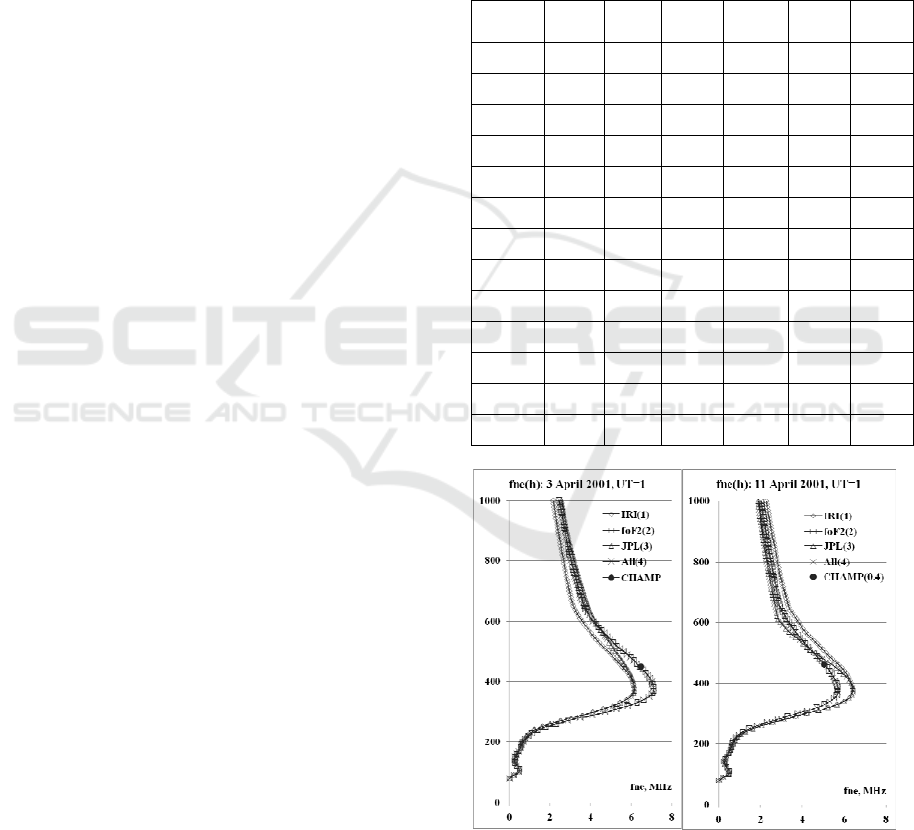
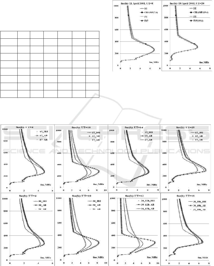
The best fit of model and the experimental
values is provided by the fourth version. Examples
of the profiles are shown in Fig. 1a, b. Fig. 1a
presents night profiles (UT=1), Fig. 1b presents
daytime profiles (UT=13). Examples for night
profiles are given for cases of foF2(obs)>foF2(IRI)
(the left panel) and foF2(obs)<foF2(IRI) (the right
panel).
Figures in round brackets after the name of the
satellite indicate a time of observation if this time
does not coincide with data of TEC. Values of the
model and satellite plasma frequencies coincide for
the forth version.
Table 2: Comparison of simulation results for different
versions of the IRI model with the data of the CHAMP
satellite
day UT
IRI
(1)
foF2
(2)
TEC
(3)
All
(4)
CH
fne
3 1 5.57 6.45 5.75 6.44 6.50
3 13.1 9.27 10.70 10.14 10.94 11.14
6 12.6 9.33 9.97 9.84 10.15 10.01
11 0.4 5.72 5.07 5.41 5.06 5.04
13 12.6 9.16 11.09 9.96 10.87 11.16
19 23 6.51 5.02 5.07 4.92 4.37
21 23.2 6.52 6.53 6.45 6.46 6.21
23 23.4 6.52 5.80 5.91 5.67 5.35
24 22.7 6.53 6.15 6.30 6.11 6.00
26 22.9 6.53 6.53 6.55 6.55 6.92
29 11.2 8.14 8.88 8.60 8.65 8.74
29 22.5 6.54 5.85 6.04 5.78 5.74
30 10.5 8.10 8.05 8.21 8.20 7.76
Figure 1a: Comparison of model Ne(h)-profiles and the
results for the CHAMP satellite (April 2001) for night
time
A New Model of The International Reference Ionosphere IRI for Telecommunication and Navigation Systems
131

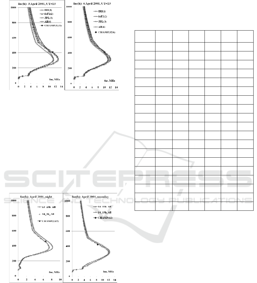
Figure 1b: Comparison of model Ne(h)-profiles and the
results for the CHAMP satellite (April 2001) for day time
The same correspondence can be seen for the
noon time profiles, although the time of the satellite
flight is slightly different from the time of
measurement of ionospheric parameters. Exact
coincidence of these times is rare.
More often are the cases when the satellite
passed over the station at even hours, whereas the
values of TEC were only for the odd hours. Typical
examples of calculations for these cases are shown
in Fig. 2 for daytime and nighttime profiles for the
forth option (full adjustment).
Figure 2: The cases of the satellite flight in the average
hours between the measurements of the TEC
Orbit heights of DMSP satellites exceed 800
km.The results using data of DMSP were obtained
under the same scenario. In this case data of three
satellites were available (F12, F13, F15). Typical
results are shown in the Table 3. They present
plasma frequencies for four options and
experimental values fne.
Table 3: Comparison of simulation results for different
versions of the IRI model with data of DMSP satellites
(hsat~840-860 km)
day UT
IRI
(1)
foF2
(2)
JPL
(3)
All
(4)
fne
1 5.5 2.10 1.22 1.71 2.07 2.15
1 8.7 3.46 2.73 2.88 3.40 2.71
1 15.3 3.32 3.17 3.67 3.76 3.36
1 17.4 3.10 2.95 3.61 3.67 3.02
2 5.3 2.13 2.13 2.77 2.77 2.38
2 7.5 2.76 3.00 3.74 3.62 2.94
2 17.2 3.11 3.41 3.77 3.61 2.75
3 7.3 2.77 3.28 4.06 3.79 2.89
3 8.2 3.47 4.03 4.68 4.35 3.41
3 16.5 3.15 3.69 4.20 3.92 3.33
4 4.9 2.15 2.73 3.44 3.22 2.76
4 7 2.77 3.17 3.97 3.77 3.04
4 19.4 2.96 3.38 3.89 3.70 3.44
5 19.2 2.97 2.87 3.31 3.35 2.81
11 19.4 3.04 3.60 3.60 3.27 3.52
12 4.8 2.23 1.39 1.38 1.95 1.73
12 7 2.82 1.69 1.93 2.64 2.19
12 19.2 3.05 2.75 2.45 2.68 1.60
13 4.6 2.24 2.08 2.19 2.29 1.80
The distinction
of this case is the fact that the best
agreement between the calculated and experimental
values of fne is obtained for the original model or
adaption of the model to current foF2. Using the
experimental values of TEC leads to
overvalued
values of fne. A too high value for the map of JPL
should be considered as a possible cause. This can
be confirmed by the results for other maps presented
in Fig. 3. Experimental plasma frequencies fne are
shown by full points, the other values are
corresponding to various maps.
It is seen that often experimental frequencies do
not reach range of map values. Nevertheless, the
agreement between the calculated and experimental
values of fne exists. Typical examples of Ne(h)-
profiles are shown in Fig. 4 as close to the moment
of the flight time and for the middle of two hour
period.
First International Conference on Telecommunications and Remote Sensing
132

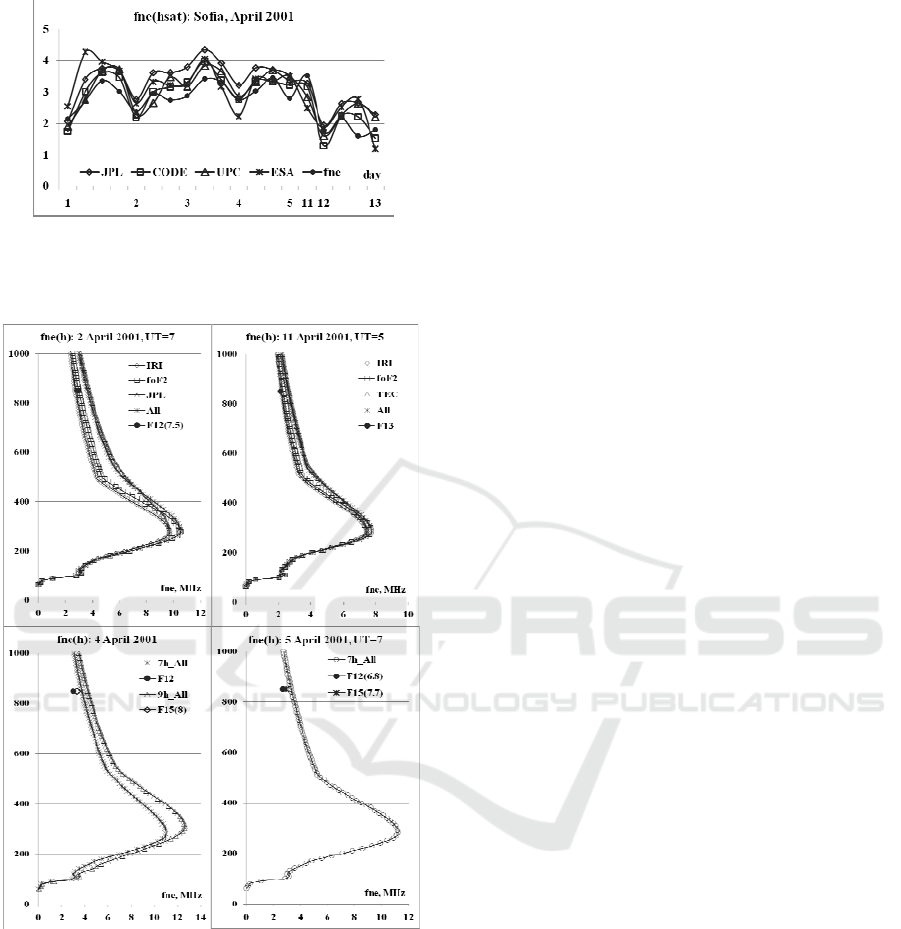
Figure 3: Comparison of experimental plasma frequencies
fne and frequencies provided by maps of JPL, CODE,
UPC, ESA
Figure 4: Comparison of model Ne(h)-profiles and the
results of the DMSP satellite (April 2001)
5 EXAMPLES OF THE
BEHAVIOR OF Ne(h)-
PROFILES AT THE SOFIA
STATION DURING
DISTURBANCES
The results of the previous section show that the
profiles are rather well adapted to meet the satellite
measurements. This allows us to study and simulate
the height distribution of the ionospheric ionization.
The choice of Ne(h)-profiles in the previous section
was dictated by time of flight of the satellite. For a
variety of tasks long periods of observation are
important especially for disturbed conditions when
the profiles can be strongly modified. Examples of
the behavior of Ne(h)-profiles for the longitudinal
(left panels) and latitudinal (right panels) chains
connected with the Sofia station are shown in Fig.
5.The upper two sets of graphs display night profiles
(UT = 1), the bottom two groups – daytime profiles
(UT=11). The upper graphs of each group show the
profiles during quiet conditions, the lower profiles -
in the disturbed ones. In the night of 12 April, quiet
conditions on the longitudinal chain (Sodankyla,
Leningrad, Moscow, Sofia) are presented by Ne(h)-
profiles of the IRI model. We can see the
coincidence of the values of three northern stations
and high values for Sofia because it is the most
southerly. During the disturbance, which is negative,
the profiles vary strongly, because all the
ionospheric structures are shifted to the south. Thus,
the Moscow station is in the area of the ionospheric
trough, the Leningrad station falls from the
plasmaspheric area into zone of subauroral
amplification. The most strongly reduced is the
concentration at the Sofia station reaching values
less even than the values in the subauroral
Sodankylä station. This leads to huge gradients of
the electron concentration that must be considered in
the propagation of radio waves. On the latitudinal
chain (Sofia, Rome, Ebre), profiles of the Sofia
station have the lowest ionization, indicating a
positive gradient towards lower latitudes under quiet
conditions. During the negative disturbance, a
decrease in the concentration at all the stations can
reduce gradients. During the day, the concentration
distribution in the quiet time should be clearly
decreased with increasing latitude. An example of
the lower grafts shows that a positive (in this case)
perturbation has the greatest effect on the
concentration of the Sofia station. Example of
daytime profiles for a quiet state and during the
April 3 disturbance is shown in the lower right-hand
chart. It is seen that if a negative disturbance during
the night enveloped almost the entire European
region, the daytime disturbance may influence by
different manner at various stations.
Since the bottom and topside parts of the profile
may respond differently to disturbance, such profiles
can provide a quantitative assessment of effects of
disturbances.
A New Model of The International Reference Ionosphere IRI for Telecommunication and Navigation Systems
133

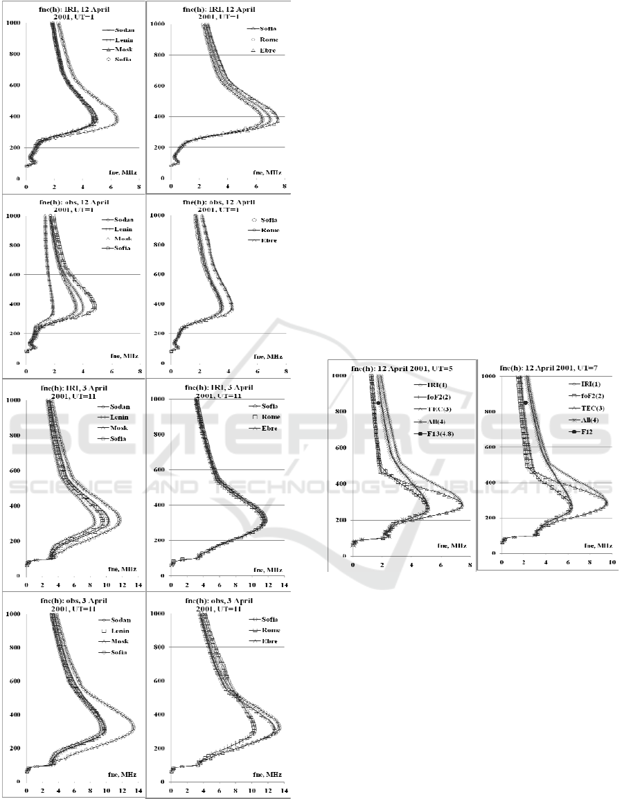
Figure 5: Sequence of Ne(h)-profiles showing their
modification during the disturbances
6 CASES OF LACK OF
MEASUREMENT OF
IONOSPHERIC
PARAMETERS AT THE
STATION
In the absence of measurements of ionospheric
parameters at the station there are at least two
methods to obtain Ne(h)-profiles: (1) the use of the
parameters of the original model, (2) the use of the
median equivalent thickness of the ionosphere
τ(med) in conjunction with the TEC. The first option
coincides with the first option of the section 4 and
provides good results for the conditions close to the
quiet ones, but during the disturbances difference
can be substantial, as illustrated in Fig. 6. Fig. 6
shows the results of calculations for all versions. It is
evident that the difference is significant, not only
near the peak of the layer F2, but at the top of the
profile. The full points indicate the plasma
frequency of DMSP satellites.
Figure 6: Comparison of Ne(h)-profiles in the case of
strong differences in foF2 (IRI) and foF2 (obs), caused by
a disturbance
These two successive profiles show an increase
in the diurnal foF2, but the perturbation has a strong
influence. Therefore, it is preferable to use the
second method. In (Maltseva et al., 2012) is shown
that the use of the median equivalent thickness of the
ionosphere τ(med) in conjunction with the TEC
allows us to fill in gaps in the data by means of
using reconstructed values of foF2. The
effectiveness of this approach is estimated using the
deviations of the calculated and experimental values
of foF2 for periods when there are complete data
sets. For four disturbed periods in April 2001 for the
Sofia station, these deviations are shown in Fig. 7.
First International Conference on Telecommunications and Remote Sensing
134

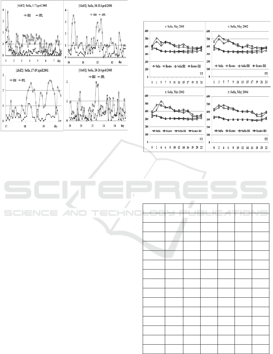
Figure 7: Deviations of the model and reconstructed
values of foF2 from the experimental ones
It is seen that the greatest deviations of model foF2
values from the experimental ones account for the
days of disturbances. Using τ(med) in conjunction
with the TEC can increase compliance by many
times. This section contains attempts to do the next
step: to use τ(med) of one (reference) stations for the
determination of foF2 of another station from its
values of TEC. We validate this procedure with the
help of satellite data. The results are shown in the
example of May 2005, which was also marked by
four disturbances with minimal index Dst:-127nT
(8.05), -263nT (15.05), -103nT (20.5), -138nT
(30.5). For the Sofia station, ionospheric observation
data are absent in the SPIDR database since 2005.
Rostov was chosen as the reference station to
determine the values of foF2 for the Sofia station.
Values of τ(med) of the Rostov station and TEC
values of the Sofia station are used. To be sure in
correctness of using τ(med) of the Rostov station we
compared τ(med) of these stations for some previous
years. Fig. 8 displays experimental and model values
of median equivalent thickness τ of the ionosphere
for stations of Sofia and Rostov in May of those
years for which measurements were available
simultaneously at both stations in the SPIDR. Model
values (sign IRI) shown by the triangles and
asterisks coincide. Namely these values are used in
traditional methods of determining foF2 from TEC
(McNamara, 1985; Houminer and Soicher, 1996,
Gulyaeva, 2003). They ensure deviations between
experimental and model values of foF2 shown in
Fig. 7 by circles. The more important fact is the
closeness of the experimental values of τ(med) for
both stations. Using these values ensures deviations
shown in Fig. 7 by points.
Figure 8: Comparison of equivalent thicknesses τ for Sofia
station
Table 4: Comparison of simulation results for different
versions of the IRI model with the data of CHAMP
satellite in May 2005 (hsat~860 km)
day UT IRI foF2 TEC All fne
1 9 5.73 5.69 5.95 5.93 5.41
2 21.3 4.82 3.67 4.76 3.70 3.91
3 8.4 4.99 5.33 5.48 5.65 5.45
4 20.7 5.69 5.31 5.66 5.34 3.99
6 8.3 4.97 5.33 5.47 5.65 4.59
12 8 4.91 5.34 5.44 5.66 4.55
12 19.9 5.87 5.97 5.99 6.07 6.02
18 19.6 5.96 5.08 5.77 5.15 4.87
21 19.5 5.97 5.38 5.93 5.48 5.27
23 7.1 4.88 4.97 5.26 5.30 3.81
24 19.3 5.99 5.83 6.09 5.95 5.78
28 6.3 4.65 5.59 5.34 5.93 5.46
28 18.5 6.07 6.45 6.41 6.72 6.55
29 18.6 6.06 6.38 6.39 6.65 7.05
30 5.7 4.65 4.48 4.89 4.81 4.07
The profiles obtained using the reconstructed values
of foF2 are compared with data of CHAMP and
A New Model of The International Reference Ionosphere IRI for Telecommunication and Navigation Systems
135

DMSP satellites. The results are shown in Tables 4-5
separately for each satellite. In this case, there were
more flights with similar times for both satellites, so
in the Table 5 we focus on the close passages.
Table 5: Comparison of simulation results for different
versions of the IRI model with data of DMSP satellites in
May 2005 (hsat~840 km).
day UT IRI foF2 TEC All fne
1 7.2 1.89 1.99 2.33 2.29 1.81
3 8.4 1.88 1.99 2.33 2.28 1.61
4 19.6 1.91 1.79 1.81 1.90 1.12
6 6.2 1.85 1.97 2.30 2.26 1.48
18 19.4 1.93 1.66 1.61 1.84 1.18
23 5.3 1.77 1.82 2.14 2.12 1.46
29 18.2 1.92 2.02 2.52 2.46 1.58
30 5.3 1.77 1.71 1.96 1.99 1.48
The results are very similar to the results for April
2001, indicating the effectiveness of this approach.
The proximity of the flight time allowed us to
compare Ne(h)-profiles adapted to the values of
plasma frequencies for both satellites. Examples of
such profiles are shown in Fig. 9.
Figure 9: Examples of Ne(h)-profiles adapted to the data
of both satellites
An important result is the fact that adaptation to
data of various satellites leads to almost the same
profile. This suggests that the behavior of the
profiles will reflect the real situation. An example of
the behavior of profiles during two disturbances in
May 2005 is shown in Fig. 10.
Figure 10: The behavior of the Ne(h)-profiles of the Sofia station during two disturbances in May 2005
First International Conference on Telecommunications and Remote Sensing
136

Surprising is the identity of changes during these
two disturbances, which may indicate some
regularities. IRI profiles correspond to quiet
conditions. Comparison with these profiles shows
that in the early morning hours (UT = 4) on 15 and
30 May at the bottom, the ionosphere is close to the
quiet state, and in the topside there is an increase of
ionization. On 17 and 31 May, a decrease in the
bottom part is observed along with an increase at the
topside. This demonstrates the different responses of
the upper and lower parts of the ionosphere on the
disturbance. In moments of UT = 10 both
disturbances are manifested in the form of large
increases in the bottom part and the weakening of
the ionization at the topside. On May 30 at UT = 12,
this process is developing at the time, as on 15 May
(chart is not shown), it decays. In UT = 18, both the
profiles return back to its original state.
7 REFINEMENT OF THE TEC
VALUES FROM SATELLITE
EXPERIMENTS
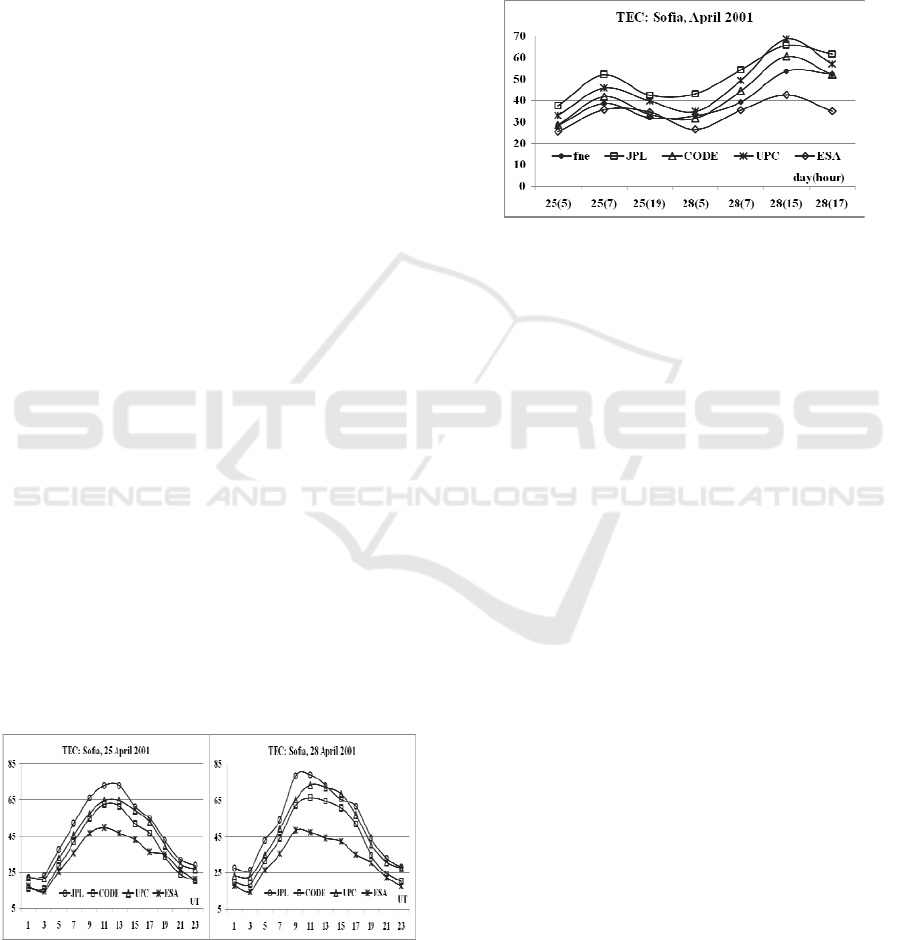
Figure 3 shows that there is some variation in
correspondence related to the difference in TEC.
The difference of the TEC values related to one
point and one moment of time is a known fact. The
reasons for the differences may be very different.
For global maps of JPL (Mannucci et al., 1998),
CODE (Schaer et al., 1995), UPC (Hernandez-
Pajares et al., 1999), ESA (Sardon et al., 1994;
Jakowski et al., 1996), it is the difference in
calculation methods. Various receivers may give
difference of up to 10 TECU (e.g. Choi et al., 2010).
A typical example is Figure 7 of the article (Arikan
et al., 2003), which shows the values of TEC,
obtained by different methods in the Kiruna station
on 25 and 28 April 2001. The values of the global
maps for the Sofia station for these two days are
shown in Fig. 11.
Figure 11: Differences of TEC for the Sofia station
calculated from the various global maps
It is seen that the difference in the Sofia station
for four maps may lie in the range of 10-30 TECU.
In this paper is proposed to specify these values
using the plasma frequency on satellites. Fig. 12
shows the values of TEC for four maps and the
values obtained by adapting the model to fne on
satellites. In the abscissa, day and hour of
calculations are indicated.
Figure 12: Comparison of TEC calculated from the
various global maps with TEC obtained by adaptation to
the satellite fne
It is seen that the values of the JPL map are
overvalued. It is possible that such adaptation can be
used to calibrate the TEC for a given station.
8 CONCLUSIONS
The ionosphere is the key factor for the operation of
satellite systems. It is one of the largest sources of
error in positioning and navigation. The associated
error is proportional to the TEC. That is why a lot of
attention paid to the development of the ionospheric
model. Using the model of Klobuchar (e.g. 1987)
allowed to increase the positioning accuracy in 2
times. The next step was done using the IRI model.
However, the previous versions of this model also
had limitations. This paper highlights the
possibilities of a new model (Gulyaeva et al., 2002;
Gulyaeva, 2003). They confine to the fact that
adaptation of the IRI model to current ionospheric
parameters foF2, hmF2 and TEC allows us to
determine the state of the ionosphere up to altitudes
of high-altitude satellites with greater accuracy than
ever before. The use of plasma frequency fne,
measured at altitudes of satellites, on the one hand,
allows us to validate the model and determine the
behavior of the Ne(h)-profiles, on the other hand,
may provide
refinement of TEC values which
depend on the accuracy of satellite systems from.
According to data of the Sofia station, effectiveness
of the use of the median equivalent thickness of the
A New Model of The International Reference Ionosphere IRI for Telecommunication and Navigation Systems
137

ionosphere τ (med) is confirmed not only to fill gaps
of foF2 at one station, but also to determine the
behavior of foF2 for the other stations in the absence
of its experimental data.
ACKNOWLEDGEMENTS
Authors thank scientists provided data of SPIDR,
global maps of TEC, operation and modification of
the IRI model, Dr A. Karpachev for CHAMP data.
REFERENCES
Araujo-Pradere, E.A., Fuller- Rowell, T.J., Bilitza, D.,
2004. Time Empirical Ionospheric Correction Model
(STORM) response in IRI2000 and challenges for
empirical modeling in the future. Radio Sci. 39,
RS1S24, doi:10.1029/2002RS002805.
Arikan, F., Erol, C. B., Arikan, O., 2003. Regularized
estimation of vertical total electron content from
Global Positioning System data. J. Geophys. Res. 108
(A12), 1469, doi:10.1029/2002JA009605.
Bilitza, D., 2001. International Reference Ionosphere.
Radio Sci. 36 (2), 261-275.
Bilitza, D., 2006. The International Reference Ionosphere
– Climatological Standard for the Ionosphere. In
Characterising the Ionosphere (pp. 32-1 – 32-12).
Meeting Proceedings RTO-MP-IST-056, Paper 32.
Neuilly-sur-Seine, France: RTO. Available from:
http://www.rto.nato.int/abstracts.asp.
Bilitza, D.,
2009. Evaluation of the IRI-2007 Model
Options for Topside Electron Density, Adv. Space
Res., 44(6), 701–706.
Bilitza, D., Reinisch, B.W., 2008. International Reference
Ionosphere 2007: Improvements and New Parameters.
Adv. Space Res. 42. 599-609.
Bilitza, D., Reinisch, B.W., Gulyaeva, T., 2010.ISO
technical specification for the ionosphere – IRI recent
activities. In Report presented for COSPAR Scientific
Assembly, Bremen, Germany, C01-0004-10.
Choi, B.-K., Chung, J.-K., Cho, J.-H., 2010. Receiver
DCB estimation and analysis by types of GPS
receiver. J. Astron. Space Sci., 27(2), 123-128.
Gulyaeva, T.L., 2003. International standard model of the
Earth’s ionosphere and plasmasphere. Astronomical
and Astrophysical Transactions. 22(4), 639-643.
Gulyaeva, T.L., Huang, X., Reinisch, B.W., 2002.
Ionosphere-plasmasphere software for ISO. Acta
Geod. Geoph. Hung. 37, 143-152.
Hernandez-Pajares, M., Juan, J.M., Sanz, J., 1999. New
approaches in global ionospheric determination using
ground GPS data. J. Atmos. Sol. Terr. Phys., 61, 1237–
1247.
Houminer, Z., Soicher, H., 1996. Improved short –term
predictions of foF2 using GPS time delay
measurements. Radio Sci. 31 (5), 1099-1108.
Jakowski, N., Sardon, E., Engler, E., Jungstand, A., Klahn,
D., 1996. Relationships between GPS-signal
propagation errors and EISCAT observations. Ann.
Geophys., 14, 1429-1436.
Klobuchar, J.A., 1987. Ionospheric time-delay algorithm
for single-frequency GPS users. IEEE Transactions on
aerospace and electronic systems. AES-23(3), 325-
331.
Maltseva, O.A., Mozhaeva, N.S., Poltavsky, O.S.,
Zhbakov, G.A., 2012. Use of TEC global maps and
the IRI model to study ionospheric response to
geomagnetic disturbances. Adv. Space Res. 49, 1076-
1087.
Maltseva, O.A., Zhbankov, G.A., Nikitenko, T.V., 2011.
Effectiveness of Using Correcting Multipliers in
Calculations of the Total Electron Content according
to the IRI2007 Model. Geomagnetism and Aeronomy,
51(4), 492–500.
Mannucci, A. J., Wilson, B. D., Yuan, D. N., Ho, C. H.,
Lindqwister, U. J., Runge, T. F., 1998. A global
mapping technique for GPS-derived ionospheric total
electron content measurements. Radio Science, 33(3),
565-582.
McNamara, L.F., 1985. The use of total electron density
measurements to validate empirical models of the
ionosphere. Adv. Space Res. 5(7), 81-90.
Sardon, E., Rius, A., Zarraoa, N., 1994. Estimation of
the receiver differential biases and the ionospheric
total electron content from Global Positioning System
observations. Radio Sci., 29, 577-586.
Schaer, S., Beutler, G., Mervart, L., Rothacher, M.,
Wild, U., 1995. Global and regional ionosphere
models using the GPS double difference phase
observable. In IGS Workshop, Potsdam, Germany,
May 15-17, 1-16.
Stankov, S.M., Jakowski, N., Heise, S., Muhtarov,
P.,Kutiev, I., Warnant, R., 2003. A New Method for
Reconstruction of the Vertical Electron Density
Distribution in the Upper Ionosphere and
Plasmasphere. J. Geophys.Res., 108, 1164;
doi:1029/2002JA009570.
Uemoto, J., Ono, T., Kumamoto, A., Iizima, M., 2007.
Comparison of the IRI 2001 Model with Electron
Density Profiles Observed from Topside Sounder
On_Boardthe Ohzora (EXOS_C) and the Akebono
(EXOS_D) Satellites, Adv. Space Res., 39(5), 750–
754.
Zhang, S.-R., Holt, J.M., Bilitza, D., van Eykan, T.,
McCready, M., Amazory-Mazaudier, C., Fukao, S.,
Sulzer, M. 2007. Multiple-site comparisons between
models of incoherent scatter radar and IRI Adv. Space
Res. 39. 910-917.
First International Conference on Telecommunications and Remote Sensing
138