
SOME EFFECTS OF THE ASSUMPTION OF ALL-POLE FILTER,
USED TO DESCRIBE PROCESSES OF TYPE “PULSE SOURSE -
FILTER”, ON THE PROPERTIES OF THE GENERATD SIGNAL
Damyan Damyanov, Vassil Galabov
Technical University of Sofia, Faculty of Automation, Department for Industrial Automation,
Bulgaria, Sofia, Darvenitsa 1756,Bul. Kliment Ohridksi 8, block 9,rooms 9416 and 9420
damyan.damyanov@fdiba.tu-sofia.bg , vtg@tu-sofia.bg
Keywords: “pulse source – filter” model of speech production, speech communication in control systems.
Abstract: In practice, when analysing, processing and generating signals, it is often assumed, that the process is of
type “pulse source - filter”. Examples include the speech production process according to the theory of Fant,
analysis of shockwaves, ECG, EEG, seismology. For determination of the parameters of the filter many
methods exist, most of which require the assumption of linear, all-pole model of the filter. It dates from the
time when the computational power of the processing systems was very low. From the 50-s on, many
computational effective algorithms have been created. Their complexity is almost an order smaller
compared to those, using other models of the filter. In frequency domain the all-pole filter describes very
well the processes, for which it has been created. In most of the practical solutions it has became classics,
and what follows is his application for other purposes, for which it may be inappropriate. In this paper, some
general properties in the application of linear all-pole filter and pulse-source for generating of periodical
signal are reviewed. These properties explain some phenomena of the modelled real process and give better
interpretation for the constraints, which come out from the implementation of such model.
1 INTRODUCTION
A “pulse source – filter” model could be represented
as shown on fig.1:
Figure 1: A “pulse source – filter” model.
The observed signal S(s) is defined by the
parameters of the filter H(s), excitation pulses E(s)
and by the noise Z(s) (Fant G., 1990. In practice
statistical methods of autocorrelation and
autocovariation are used (Epsy-Willson et.al, 2006,
Prasana, S., et.al, 2006). If for sake of clarity we
don’t take into account the additive input noise, the
generation of the signal in z-domain could be written
as:
nTt
tsnTsnTsZzS
zHzEzS
=
==
(1)
=
)()()},({)(
)()()(
Without ignoring the importance of the derived
conclusions, we can assume H(z) as a all-pole filter
(Titze, 1984):
(2)
∑
=
−
+
=
M
i
i
i
za
zH
1
1
1
)(
139
Damyanov D. and Galabov V.
SOME EFFECTS OF THE ASSUMPTION OF ALL-POLE FILTER, USED TO DESCRIBE PROCESSES OF TYPE "PULSE SOURSE - FILTER", ON THE PROPERTIES OF THE GENERATD
SIGNAL.
DOI: 10.5220/0005415101390145
In Proceedings of the First International Conference on Telecommunications and Remote Sensing (ICTRS 2012), pages 139-145
ISBN: 978-989-8565-28-0
Copyright
c
2012 by SCITEPRESS – Science and Technology Publications, Lda. All rights reserved

The problem of finding the coefficients of the
filter
,=1,
can be defined as signal analysis.
If the input of the filter with transfer function H(z) is
a delta impulse, the output will be an envelope of a
signal element, modelled with the current filter
coefficients. The model of the signal analysis:
(
)
=
(
)
(
)
(3)
uses a filter, inverse with the exciting one, with
transfer function:
(
)
=
1
(
)
=
1
+
(4)
Two approaches for finding of the coefficients of the
filter are possible – assuming asynchronous
excitation, and assuming synchronous one. The first
one assumes that the length of the analysed
quasistationary intervals is set and known apriory,
and the second assumes that the length of the
analysed quasistationary intervals is multiple of the
of the excitation period.
The method of linear prediction of M-th order
(Wiener, 1966) approximates the current value of
the signal () from a discrete time series
{
()
}
with a linear combination of M preceding values
with the corresponding weighting coefficients
:
̂
(
)
=
(
−
1
)
(
5
)
The prediction error is:
(
)
=
(
)
−
̂
(
)
(6)
For a signal segment, containing N samples, the
weighting coefficients can be optimized in such
way, that the sum of squares of the errors of
prediction for all N samples is minimal. In this case
the objective function for the optimization is:
(
)
=
(
)
−
(
−
)
!
=
(7)
Setting the partial derivative of the sum of
squares equal to zero we have the equation:
(
−
)
(
−
)
=
(
)
(
−
)
,
=
1
,
(8)
Two common methods, differing in the limits of
summation are known: autocorrelation and
autocovariation.
The range of summation of the autocorrelation is
−∞<<∞ :
Φ
(
|
−
|
)
=
Φ
(
)
,
=
1
,
(9)
with the coefficients of autocorrelation :
Φ
(
|
−
|
)
=
(
−
)
(
−
)
(
10
)
The interval to be analysed is actually 0<<,
the samples outside it could be eliminated with an
appropriate window function (), and the
autocorrelation coefficients (), can be evaluated
as follows:
(
)
=
(
)
(
+
)
,
(
)
=
(
)
(
)
,
(
)
=
≠0,0≤<
0
=
0
.
(11)
The equality from the condition for unconditional
optimization becomes:
(
|
−
|
)
=
(
)
,
=
1
,
(12)
and as a matrix notation:
(
,
,
…
,
)
=
(
(
1
)
,
(
2
)
,
…
,
(
)
)
(1
3
)
The matrix R of the coefficients (
|
−
|
) is a
Toeplitz matrix – it is symmetrical and the elements
in the diagonals are identical (Grenader. U. et. al. ,
1958) :
First International Conference on Telecommunications and Remote Sensing
140

=
⎝
⎜
⎜
⎜
⎛
R
(
0
)
R
(
1
)
⋯
R
(
M
−
1
)
R
(
1
)
R
(
0
)
⋯
R
(
M
−
2
)
R
(
2
)
R
(
1
)
⋯R
(
M−3
)
⋯
⋯
⋯
⋯
R
(
M
−
1
)
R
(
M
−
2
)
⋯
R
(
0
)
⎠
⎟
⎟
⎟
⎞
(14)
There are a lot of methods for solving the system
of equations. The most effective is the recursive
method of Durbin, where the number of operations
grows only with the square of the weighting
coefficients (Makhoul, J., 1975).
Because their value is always less than one, the
poles of the filter will always be within the unit
circle on the z-plane, which guaranties its stability.
When using the covariation, the prediction error is
minimized within the interval 0<< . The
matrix of the coefficients in general isn’t a Toepliz
one and the methods for obtaining the filter
coefficients aren’t so effective (the Cholesky method
for example (Werner, H, 1975)) and the stability of
the filter isn’t guaranteed.
Both the autocorrelation and covariation use the
same two steps for evaluating the filter coefficients.
– first they find the coefficients matrix, and then
solve the system of linear equations (Madisetti V.,
Williams D, 1999). There are other possible
methods, (for example using lattice structures),
which combine the two steps. In can be proven
(Makhoul, J., 1975) that the most effective method is
the one of Durbin, which is the most preferred
autocorrelation method.
2 IMPACT OF THE DURATION
OF THE EXCITATION PHASE
TO THE PERIOD OF THE
SPECTRAL PEAK
We assume model of the filter is of order two:
(
)
=
+
(15)
This means that the signal will contain only one
spectral peak
. If the filter is excited by a
sequence of rectangular pulses, described by:
(
)
=
1
,
(
−
1
)
≤
<
excitation
_
phase
+
(
−
1
)
0
,
excitation
_
phase
+
(
−
1
)
≤
<
=
1
,
−
1
(16)
Where
is the excitation period, and
_
is the duration of the excitation
phase. The output signal for the first excitation
period (m=1) is:
_
(
)
=
_
−
_
sin
(
+
_
)
(17)
for <
_
, i.e. in excitation phase,
and:
_
(
)
=
_
sin
(
+
_
)
(18)
for ≥
_
, i.e. in free vibration
phase, where:
_
=
is the constant component of
the signal in the excitation phase
_
=
and
_
=2
sin(
_
) are the
amplitudes of the signal in excitation phase and in
the phase of free vibration
_
=
and
_
= 2−
_
are the
angular phases of the signal in excitation phase and
in the phase of free vibration
=2
are the circular frequency, which
corresponds to the spectral peak
.
We can observe the following:
§ The amplitude of the signal in th excitation
phase depends only on the gain constant of
the filter
§ The amplitude of the signal in the phase of
free vibration depends again on the gain
constant, but also in a complicated way on
the ratio of duration of the preceding phase
of excitation to the period of the spectral
peak.
§ The later holds true also for the angular
phases.
This means that changes in the duration of the
excitation phase can increase or decrease the
amplitudes of the spectral peaks , without changing
the parameters of the filter. To illustrate this impact,
we define a dimensionless coefficient, proportional
to the ratio of duration of the excitation phase to the
period of the spectral peak :
_
=
_
(19)
Some Effects of the Assumption of All-Pole Filter, Used to Describe Processes of Type "Pulse Sourse -
Filter", on The Properties of the Generatd Signal
141
For the relation of the amplitudes of the signal in
the excitation phase and in the phase of free
vibration we define the coefficient:
_
_
=
_
_
(
20
)
Here
_
=
−
_
means
the duration of the free vibration phase of one
excitation period. The relation between these
coefficients is:
_
_
=
2
sin
(
_
2
)
(21)
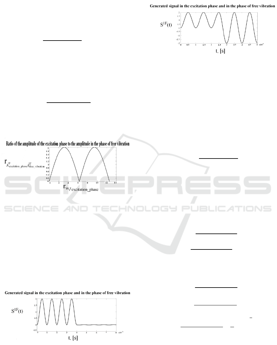
Obviously this relation is periodical, and the first
two periods are shown in fig.2
Figure 2: The relation of the amplitude of the generated
signal in the excitation phase to the amplitude of the phase
of free vibration as function of the coefficient
_
.
As one can see, varying the duration of the
excitation phase, without changing the filter
coefficients, the amplitude of the spectral peak of the
generated signal in the free vibration phase can take
any value from zero (fig.3) to two times the
amplitude in the excitation phase (fig.4).
Figure 3: The generated signal in the excitation phase and
in the phase of free vibration with
_
=2,=0,±1,±2…. and
excitation_phase
free_vibration
=0
Figure 4: The generated signal in the excitation phase and
in the phase of free vibration with
_
=,=±1,±3…. and
excitation_phase
free_vibration
=2
This effect becomes more apparent within a
signal segment, containing more than one excitation
period. In this case not only the coefficient
_
, but also the ratio of the duration
of the excitation phase to the excitation period,
which is actually the is mark-to-space ratio, will be
of importance for the ratio of the amplitudes:
_
=
_
(22)
The derived analytical relations lead us to important
conclusions. The ratio of the amplitudes of the signal
in the excitation phase to the phase of free vibration
for the second excitation period is given by the
relation:
_
_
=
⎣
⎢
⎢
⎢
⎡
4
sin
1
_
2
cos
1
_
2
⎦
⎥
⎥
⎥
⎤
sin
_
+
sin
2−
_
+
−2
sin
_
2
+
sin
_
−
2
(2
3
)
The graphical representation of this relation is
shown in fig 5.
Obviously for the next periods the calculation of this
ratio is getting more and more complicated and
First International Conference on Telecommunications and Remote Sensing
142

some numerical methods are needed. Nevertheless,
the following important observation can be made:
Figure 5: The relation of the amplitudes of the generated
signal in the excitation phase to the phase of free vibration
for the second excitation period.
Varying the ratio of the duration of the excitation
phase to the duration of the period of excitation, and
without changing the parameters of the filter, one
can generate segments, in which the amplitude of the
spectral peak for every following period of
excitation increases, decreases, doesn’t change
considerably, or follows some analytical relation.
3 IMPACT OF THE DURATION
OF THE EXCITATION PHASE
WITH MORE THAN ONE
SPECTRAL PEAK
The way, that the parameters of the excitation
change the ratio between the amplitudes of the
different spectral peaks in the generated signal, is
similar to the one, presented in the previous chapter.
We assume, that the we have all-pole filter of fourth
order, and the poles all lie of the unit circle:
(
)
=
1
(
+
)
(
+
)
(24)
If the excitation of the filter is one rectangular pulse,
the output signal will contain two spectral peaks
and
. If we assume, that
=
and
>1,
the components of the signal in the excitation phase
are:
_
(
)
=
_
−
_
sin
(
+
_
)
(
25
)
_
(
)
=
_
(26)
−
_
sin
(
+
_
)
Where:
_
=
(
)
and
_
=
(
)
are the constant
components of the first and second spectral peaks in
the excitation phase
_
=
(
)
and
_
=
(
)
are the amplitudes of the first and second
spectral peaks in the excitation phase
_
=
and
_
=
are
the angular phases of the first and second spectral
peaks in the excitation phase
=2
and
=2
are the circular
frequencies, which correspond to the spectral peaks
.and
The signal components in the phase of free vibration
are:
_
(
)
=
_
sin
(
+
_
)
(2
7
)
_
(
)
=
_
sin
(
+
_
)
(2
8
)
Where:
_
=
(
)
sin(
_
)
and
_
=
(
)
sin(
_
)
are the amplitudes of the first and second spectral
peaks in the free vibration phase
_
=−
_
is the angular
phase of the first spectral peak in the free vibration
phase
if 4≤
_
<(4+ 2) and
_
=
−
_
if
(
4+2
)
≤
< (4+ 4)
_
=−
_
is the angular
phase of the second spectral peak in the free
vibration phase
if 4≤
_
<(4+ 2) and
_
=
−
_
if
(
4+4
)
≤
<(4+ 4)
=±1,±2…
=2
and
=2
are the circular
frequencies, which correspond to the spectral peaks
.and
Some Effects of the Assumption of All-Pole Filter, Used to Describe Processes of Type "Pulse Sourse -
Filter", on The Properties of the Generatd Signal
143

As with the case with one spectral peak, we may
expect that the dimensionless coefficients,
proportional to the ratio of the duration of the
excitation phase to the period of the spectral peak
will have big influence on the parameters of the
signal components in the phase of free vibration:
_
=
_
and
_
=
_
=
_
(2
9
)
This can be represented with the dimensionless
coefficient of the ratio of the amplitudes of the two
spectral peaks in the signal
=
(
30
)
In the excitation phase this coefficient will depend
only on the filter parameters:
_
_
=
1
(
31
)
In the free vibration phase, this ratio will depend of
the filter parameters, but also in a complicated
manner on the duration of the excitation phase:
_
_
=
1
sin(
_
2
)
sin
(
_
2
)
(
3
2
)
This means, that the change of the duration of the
excitation phase can substantially change the
predetermined from filter parameters constellation of
spectral peaks in the signal. This influence can be
easily seen from the next numerical example, with
typical for a real speech signal values of the filter
parameters (Damyanov D., Galabov V., 2012):
§ First spectral peak
= 420;
§ Second spectral peak
=966; which
means
=
=2.3;
§ Nominal duration of the excitation phase
_
=2.8;
§ Fluctuation of the nominal duration of the
excitation phase ∆
_
=
±0.4;
In the excitation phase the ratio of the amplitudes
depends only on the filter parameters:
_
_
=
_
_
=
≈
0
.
189
(3
3
)
In the phase of free vibration with nominal duration
of the
_
=2.8; this coefficient
will be
_
_
≈0.288. If
the duration of the excitation phase is shortened with
4 ms, the coefficient will increase more than 20
times to
_
_
≈6.33, and if the
duration of the excitation phase is lengthened with
4ms, the coefficient will decrease more than 20
times to
_
_
≈0.061. On
fig.6 for the three cases the excitation rectangular
pulse with duration, equal to the duration of the
excitation phase, the generated signal and its spectra
are shown.
Figure 6: The three cases the excitation rectangular pulse
with duration, equal to the duration of the excitation
phase, the generated signal and its spectra.
4 CONCLUSIONS
When dealing with periodical and quasiperiodical
processes, the “source-filter” model allows
simplification of analysis and parameterization and
makes the technical implementation easier. This
facilitations can be achieved when filter and
excitation source are treated independent. In this
case for the parameterization of the filter very
efficient techniques and methods can be used. This
approach gives excellent results in most cases of use
of the model – in systems for analysis, synthesis,
coding and transmission of speech signals and
others. In some cases this description is not relevant
enough and additional complicated methods and
information sources must be used. This paper shows
that the model can be made more effective without
further complications, using the cumulative effect of
First International Conference on Telecommunications and Remote Sensing
144

simultaneous treatment of the processes, which
happen on the source and the filter.
ACKNOWLEDGEMENTS
The authors wish to thank NIS by TU-Sofia for the
financial support from contract № 122ПД0014-08,
which made this paper possible.
REFERENCES
Damyanov, D., Galabov, V., 2012, On the impact of
duration of the phase of open glottis of the spectral
characteristics if the phination process, Proceedings of
the Technical Universicty- Sofia Volume 62, Issue 2,
2012, pp. 173-180, ISSN 1311-0829
Epsy-Willson, C., Manocha, S., Vishnubholta, S., 2006, A
new set of features of text independent speaker
identification. In Proc Inter-speech 2006 (ICSLP),
Pittsburgh, Pennsylvaniq, USA, September 2006 pp.
1475-1478
Fant, G., 1990, Acoustic Theory of Speech Production,
Mouton&Co, Hauge
Granader, U., G. Szego, 1958, Toeplitz Form and Their
Applications, Berekeley CA, University of Californiq
Press, 1958
Madisetti V, Williams D., 1999, Digital Signal
Processing Handbook, New York, CRC Press, 1999
Makhoul, J, 1975, Linear Prediction: A tutorial Review,
Proceedings of the IEEE, vol. 63 1975, pp 561-580
Prasana, S., Gupta, C., Yenganarayana, B., 2006,
Extraction of speaker specific excitation information
from linear prediction residual of speech. Speech
Comm. 48, pp. 1243-1261
Titze, Ingo R., 1984, Parameterization of the glottal area,
glottal flow and the vocal fold contract area, JASA,
75(2), February, 1984, pp. 570-580
Werner, H., 1975, Praktische Mathematik, Bd. 1, Berlin
Spinger, 1975
Wiener, N., 1966, Extrapolation Interpolation and
Smoothing of Stationary Time Series, M.I.T. Press.
Cambridge, MA, 1966
Some Effects of the Assumption of All-Pole Filter, Used to Describe Processes of Type "Pulse Sourse -
Filter", on The Properties of the Generatd Signal
145
