Detection of Symmetry Points in Images

Christoph Dalitz, Regina Pohle-Fr

ohlich and Tobias Bolten

Institute for Pattern Recognition, Niederrhein University of Applied Sciences, Reinarzstr. 49, Krefeld, Germany

Keywords:

Symmetry Detection, Symmetry Transform.

Abstract:

This article proposes a new method for detecting symmetry points in images. Like other symmetry detection

algorithms, it assigns a “symmetry score” to each image point. Our symmetry measure is only based on scalar

products between gradients and is therefore both easy to implement and of low runtime complexity. Moreover,

our approach also yields the size of the symmetry region without additional computational effort. As both axial

symmetries as well as some rotational symmetries can result in a point symmetry, we propose and evaluate

different methods for identifying the rotational symmetries. We evaluate our method on two different test sets

of real world images and compare it to several other rotational symmetry detection methods.

1 INTRODUCTION

Symmetry can be a useful feature for the identiﬁca-

tion both of natural objects, like faces (Tao et al.,

2009), as well as man-made objects, like vehicles

(Kuehnle, 1991). Consequently, algorithms for de-

tecting symmetry points in images have been an area

of research for some time (Reisfeld et al., 1995) (Loy

and Zelinsky, 2003) (Loy and Eklundh, 2006) (Lee

and Liu, 2010). For a survey of symmetry detection

algorithms, see (Liu et al., 2009). All of these algo-

rithms assign each image point a “symmetry score”

that measures how well the point works as the origin

of a mirror operation. The image of symmetry score

values can then be considered as a “symmetry trans-

form” of the original image, and symmetry points cor-

respond to maxima in the symmetry transform image.

The symmetry score computation depends on the

type of symmetry. The method by Kuehnle (Kuehnle,

1991), e.g., speciﬁcally looks for vertical symmetry

axes, Reisfeld et al. (Reisfeld et al., 1995) as well as

Loy & Eklundh (Loy and Eklundh, 2006) propose dif-

ferent methods for point reﬂection or rotation symme-

try, while Loy & Zelinsky (Loy and Zelinsky, 2003)

and Lee & Liu (Lee and Liu, 2010) consider rotational

symmetry. The method proposed in the present paper

is designed for point reﬂection symmetry, which is the

same as a rotation by π around the mirror point. Let

denote the symmetry group of a rotation by an an-

gle 2π/n. Then we are looking for symmetry points of

objects with a symmetry group C

, because, when an

object is invariant under a rotation by π/m, it is also

invariant under a rotation by π.

A problem in symmetry detection is that the size

of the symmetric object is generally not known be-

forehand. For computing the symmetry score value

however, ideally only pixels belonging to the object

should be considered. The symmetry transform by

Reisfeld et al. (Reisfeld et al., 1995) requires an in-

put parameter that suppresses distant pixels exponen-

tially, which sidesteps the problem by letting the user

guess an object radius. The method by Lee & Liu

(Lee and Liu, 2010) tries a whole range of radii, but

this adds even more computational complexity to an

already very complex method. As a workaround, they

suggest the use of image pyramids so that only re-

gions that seem promising in low resolutions are ex-

amined in full detail. Our method in the present paper

offers a different solution via a recursion formula that

connects the score value for radius r +1 with the score

value for radius r, which reduces the computational

overhead of trying different radii considerably.

Another problem for the detection of rotational

symmetric objects is that, depending on the view

point, the symmetry can be “skewed” (Kanade, 1981)

(see Fig. 1(a)). Lee & Liu address this problem with a

frieze expansion around each potential rotation center

(Lee and Liu, 2010). A simpler approach with con-

siderably less computational cost can be based on the

observation that a C

symmetry approximately be-

comes a point reﬂection (C

) symmetry, provided the

object does not extend too much in the direction per-

pendicular to the image plane. In practice, rotational

symmetry will therefore generally show up as a C

symmetry, for which our method is speciﬁcally de-

signed.

577

Dalitz C., Pohle-Fröhlich R. and Bolten T..

Detection of Symmetry Points in Images.

DOI: 10.5220/0004179405770585

In Proceedings of the International Conference on Computer Vision Theory and Applications (VISAPP-2013), pages 577-585

ISBN: 978-989-8565-47-1

 2013 SCITEPRESS (Science and Technology Publications, Lda.)

(a) A C

rotational symmetry no longer holds

under distortion of perspective.

axis

rotation by

symmetry

(b) A C

rotational symmetry that also has an axial

symmetry.

Figure 1: The problems of “skewed symmetry” and axial

symmetry in rotational symmetry detection.

It should be noted however, that some pure axial

symmetries also show up as C

symmetries. A partic-

ularly frequent case are parallel lines (see Fig. 1(b)).

When detecting rotational symmetry through point re-

ﬂection symmetries, it is thus necessary to distinguish

the actual rotation symmetries from pure axial sym-

metries. In this paper we will investigate different cri-

teria for making this discrimination.

This paper is organized as follows: Sec. 2 de-

scribes the computation of our symmetry score value

and the determination of the symmetry radius. Sec. 3

describes different possible features useful for distin-

guishing high score points belonging to a rotational

symmetry from those belonging to an axial symme-

try. Sec. 4 evaluates these features on a dataset of

real world images. Moreover, the resulting symme-

try detection is compared on two different data sets to

the classic method by Reisfeld et al. (Reisfeld et al.,

1995) (Reisfeld et al., 1990) and to the newer method

by Loy & Eklundh (Loy and Eklundh, 2006), which

was reported as the best method in (Park et al., 2008)

and (Rauschert et al., 2011). In the ﬁnal Sec. 5, we

discuss open questions and make suggestions for fur-

ther research.

The source code of our symmetry transform and

the test data set with ground truth information will be

made available on the authors’ website

2 THE SYMMETRY DETECTION

METHOD

The general approach to symmetry detection consists

in ﬁrst computing a measure for the symmetry of each

http://informatik.hsnr.de/∼dalitz/data/visapp13/

(x − dx, y − dy)

(x + dx, y + dy)

(x, y)

= −

GG’

→

→→

Figure 2: Point reﬂection of an image at point (x,y) maps

the gradient

G at (x + dx,y + dy) onto the gradient

(x − dx,y − dy).

point, and then selecting points with a high symmetry

score. In this section, we deﬁne a measure for point

symmetry and show how this measure cannot only be

utilized for detecting symmetry points, but also the

size of the symmetry region.

2.1 The Symmetry Measure

Like Reisfeld et al. (Reisfeld et al., 1995), we uti-

lize the gradient image rather than the original image,

because we do not want homogeneous regions to be

recognized as symmetric. The gradient image can be

computed from a greyscale image with a Sobel ﬁlter

(Gonzalez and Woods, 2002). Let us denote the gra-

dient image with

G(x,y). When an image is mirrored

at point (x,y), the gradient

G(x +dx, y +dy) becomes

−

G(x −dx,y −dy) (see Fig. 2). We conclude that one

necessary condition for symmetry around point (x,y)

is that these two gradients point in opposite directions,

or that their scalar product h·,·i is negative:

G(x + dx,y + dy),

G(x − dx,y − dy)

< 0 (1)

This scalar product takes a minimum when the two

gradients are anti parallel. We therefore deﬁne as a

measure for the symmetry around point (x,y)

S(x,y, r) = −

∑

dy=1

∑

dx=−r

.. .

G(x + dx,y + dy),

G(x − dx,y − dy)

−

∑

dx=1

G(x + dx,y),

G(x − dx,y)

(2)

where r is the radius of the symmetry region. The

sum omits the negative values dy < 0 because these

are already taken into account by the mirror operation

in the argument of the gradient. The symmetry point

(x,y) itself is completely omitted in the sum. The mi-

nus sign is added for convenience so that S is larger

for higher symmetry, not vice versa.

It should be noted that the measure (2) does not

only take into account the gradient directions, but also

their absolute strength. This has the effect that sym-

metric regions with strong edges have a higher sym-

metry measure than regions with weaker edges, but

VISAPP2013-InternationalConferenceonComputerVisionTheoryandApplications

578

otherwise the same symmetry. One way to smooth

out this difference is by transforming the gradient

strength as suggested by Reisfeld et al. (Reisfeld

et al., 1995):

H =

· log(1 + k

Gk) (3)

and then applying (2) to

H instead of

G. Instead

of log(1 + x), any other monotonous transformation

could be used, of course. It is an open question how-

ever, whether such a rescaling actually improves the

detection of symmetry points. The experiments de-

scribed in Sec. 4 have therefore been done both with

transformed and untransformed gradients.

2.2 The Size of the Symmetry Region

When the symmetry measure S(x,y,r) according to

(2) is evaluated for different values of r, this pro-

vides a way to automatically determine the size of

the symmetry region around (x,y). Unlike the sym-

metry measure by Reisfeld et al., (2) does not in-

clude an exponential damping factor depending on a

predeﬁned region size. This means that, for a given

point (x,y), the values S(x,y,r) can be subsequently

computed for r = 1, 2,...,r

max

without any additional

computational effort, simply by reordering the sum

(2) to

S(x,y, r) = S(x,y, r − 1)

−

∑

dx=−r

G(x + dx,y + r),

G(x − dx,y − r)

−

r−1

∑

dy=−r+1

G(x + r,y + dy),

G(x − r,y − dy)

(4)

The symmetry value S(x,y) and region radius R(x,y)

for a point (x,y) can then be deﬁned as

R(x,y) = argmax{S(x,y, r) |r = 1,. .. ,r

max

}

and S(x,y) = S(x,y,R) (5)

When the region radius is close to r

max

, larger values

for r could also be tried to ﬁnd the next local max-

imum of S. This can save some computing time be-

cause large radii are then only investigated at “promis-

ing” points.

2.3 Runtime Complexity

For an image with n pixels, the Sobel ﬁlter requires

9n additions and n multiplications and is thus an O(n)

algorithm. The symmetry transform requires r

max

multiplications and additions for each pixel. As both

operations are done subsequently, the total runtime of

our symmetry transform is O(r

max

· n). Even though

this is in O-Notation the same runtime complexity as

for the symmetry transform by Reisfeld et al., our

transform is considerably faster, because it only re-

quires algebraic operations and no exponential and

trigonometric functions. Loy & Eklundh did not es-

timate the runtime complexity of their algorithm in

(Loy and Eklundh, 2006). As their algorithm does

not take all image pixels as input, but only the much

smaller set of SIFT feature points (Lowe, 2004), the

runtime complexity depends on two factors: the run-

time complexity of the SIFT extraction, and the num-

ber of SIFT points returned, which depend very much

on the image content, thereby making a worst case

runtime estimation difﬁcult.

On an Intel P8400 2.26 GHz CPU and with r

max

50, our algorithm took constantly 0.2 sec on a 200 ×

150 image from the CVPR 2011 dataset and 2.7 sec

on a 600 × 400 image from our dataset, while an op-

timized implementation (exponentials replaced with

lookup tables) of Reisfeld’s transform took about 9

sec (200 × 150, σ = 25) and 250 sec (600 × 400,

σ = 25), respectively. The runtime of Loy & Ek-

lundh’s algorithm varied considerably over the im-

ages and was between 0.3 and 1.0 sec on a 200 × 150

image, and between 1 and 18 sec on a 600 × 400 im-

age.

3 ROTATIONAL VERSUS AXIAL

SYMMETRY

As can be seen in Fig. 3, the symmetry transform de-

scribed in Sec. 2 assigns high score values to centers

of point symmetry. Some of these belong to rotational

symmetries, while others belong to axial symmetries,

mostly due to parallel strong edge lines. To discrim-

inate between these types of symmetry, we observe

that, for an axial symmetry, we obtain other sym-

metry points when moving from one symmetry point

along the symmetry axis. The same does not hold

for a purely rotational symmetry. This means that ax-

ial symmetries result in line shaped regions of high

symmetry scores, while rotational symmetries lead to

more circularly shaped regions of high symmetry. We

have therefore implemented the following three fea-

tures for determining the symmetry type of a given

candidate point (x,y):

Edge Directedness, computed on the gradient of

the symmetry transform. This measures how

“strongly directed” the edges of the symmetry

transform are. The feature is the maximum rel-

ative frequency in a histogram of the edge direc-

tions, weighted by the gradient absolute value,

DetectionofSymmetryPointsinImages

579

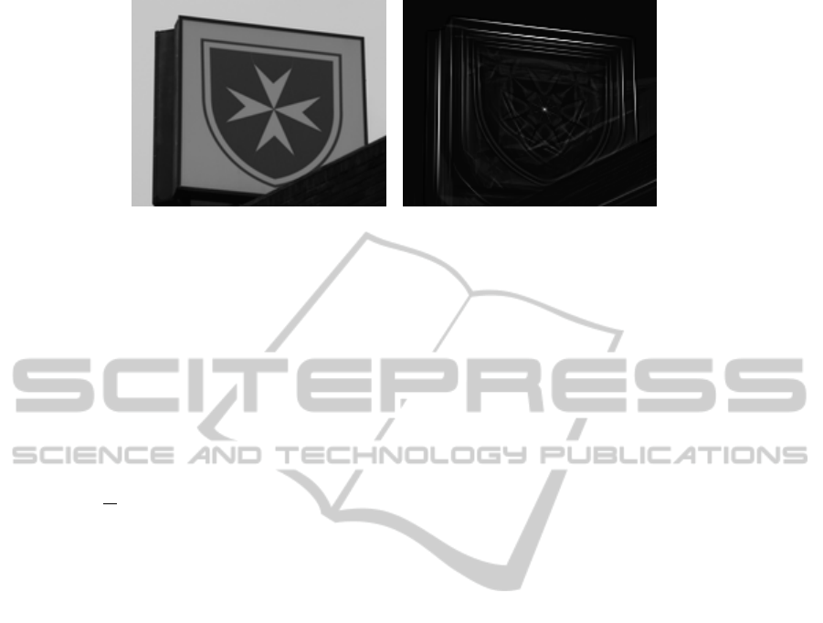
Figure 3: Symmetry transform according to Eqs. (4) and (5) of the image on the left.

in a k × k window around point (x,y). Natural

choices for the number of bins in the direction

histogram are 8 or 16. The “edge directedness”

should be higher for axial symmetries.

Covariance Eigenratio, computed on the symmetry

transform image. We compute the covariance ma-

trix K for the points in a k × k window around

(x,y) as

K =

k/2

∑

dx=−k/2

k/2

∑

dy=−k/2

S(x + dx,y + dy)



dxdx dxdy

dydx dydy



(6)

where S(x,y) is the symmetry transform value at

(x,y), and the normalization factor N is the sum

over all symmetry values in the window. The

eigenvalues of K indicate how strongly the val-

ues spread in the direction of the corresponding

eigenvector. Consequently, the ratio between the

smaller and the larger eigenvalue should be higher

for rotational symmetry, which are more isotropi-

cally spread around (x,y).

Antiparallel Directions, computed on the gradient

of the original greyscale image. We compute

the direction histogram of all gradients in a win-

dow with the symmetry radius R(x,y) according

to Eq. (5). Only those gradients are taken into

account for which the mirrored gradient is “an-

tiparallel”, i.e. the cosine of the angles between

the gradients is less than -0.975. The feature is

the highest relative frequency in the direction his-

togram. Again the number of histogram bins can

be 8 or 16. The value for “antiparallel directions”

should be lower for rotational symmetries.

In our experiments, described in Sec. 4.1, the feature

edge directedness with 16 histogram bins showed the

best performance.

4 EXPERIMENTAL RESULTS

For testing symmetry detection, there are currently

not many data sets available. Park et al. (Park et al.,

2008) selected images from different object recogni-

tion datasets for the CVPR 2008 conference, but the

resulting dataset is no longer available. At the CVPR

2011 conference, there was a workshop on symme-

try detection, and the data set, consisting of 42 im-

ages, used for evaluation is still available (Rauschert

et al., 2011). As using this data set allowed us to com-

pare our method to the other methods evaluated in this

workshop, we have used this as one of our test sets.

To allow for a more detailed investigation both of

our method and for future research, we have addi-

tionally created a new larger test set and ground truth

data. The new data set consists of 159 images of size

600×400, containing 27 different subjects. Each sub-

ject is shown in different perspectives and both in con-

text and in detail. The detail images can be useful

because, in the contextual images, the environment

often shows additional incidental symmetries. Like

Park et al. (Park et al., 2008), we have only labelled

those C

symmetries that are “visually obvious dom-

inant symmetries” according to human observers. In

the ground truth meta data, we have labelled the sym-

metry points and the radius of the symmetric region.

We have used these images both for an evaluation

of the rotational symmetry detection, and for an eval-

uation of the symmetry type discrimination. For the

latter we have created different ground truth data and

a different set of test points.

4.1 Evaluation of Symmetry Type

Discrimination

To evaluate the three features described in Sec. 3 for

discriminating between rotational and axial symmetry

points, we have selected the ten highest local maxima

in the symmetry transform of each image from our

VISAPP2013-InternationalConferenceonComputerVisionTheoryandApplications

580

0.2

0.4

0.6

0.8

0 0.2 0.4 0.6 0.8 1

false rotational symmetries

edge directedness

antiparallel directions

covariance eigenratio

true rotational symmetries

Figure 4: ROC curve comparing the performance of the

three features for discriminating between rotational and ax-

ial symmetry. “False rotational symmetries” denotes the

rate of the axial symmetries erroneously classiﬁed as rota-

tional symmetries, and “true rotational symmetries” the rate

of the correctly classiﬁed rotational symmetries.

own test set, and labeled these points manually as be-

longing to an axial or rotational symmetry. After an

omission of unclear cases, these provided a test set

of 1346 symmetry points, of which 140 belonged to

rotational symmetry.

For each feature, the classiﬁcation is based on a

threshold on the feature value. By comparing the rates

of correctly and erroneously detected rotational sym-

metries for different thresholds, we can thus compare

the discriminating power of the three features. For the

k × k windows, we have used k = 7, and as numbers

of histogram bins we have tested 8 and 16. In the case

of “edge directedness”, 16 bins were better, and for

“antiparallel directions”, 8 bins were better, i.e. had

a higher area under the ROC curve (AUC). The ROC

curves in Fig. 4 show that “edge directedness” per-

formed best on our test data. Even though the feature

“antiparallel directions” has a clearly larger AUC than

“covariance eigenratio”, it is still slightly lower than

that of “edge directedness”. As “edge directedness”

has the additional advantage of being faster to com-

pute due to the smaller window size, we have used

this feature for sorting out the axial symmetries. The

values in the upper left corner of the ROC curve cor-

respond to thresholds between 0.23 and 0.29 for the

“edge directedness”, so that we have chosen a thresh-

old of 0.27 as the criterion for rotational/axial sym-

metry discrimination in Sec. 4.2.

4.2 Evaluation of Rotational Symmetry

Detection

To compare a new method with other methods for ro-

tational symmetry detection, there are principally two

approaches: one is to implement and run the different

algorithms on a new test set, the other one is to run the

new algorithm on an older data set for which results

have already been reported in an earlier study. For the

latter approach, we have used the CVPR 2011 data

set (Rauschert et al., 2011). For the former approach,

we have deployed the code published by Loy & Ek-

lundh on their website (Loy and Eklundh, 2006), and

have additionally implemented ourselves the classic

method by Reisfeld et al. (Reisfeld et al., 1995).

Concerning the latter algorithm, it should be noted

that Reisfeld at al. gave different formulas for the ro-

tational symmetry score in (Reisfeld et al., 1990) and

(Reisfeld et al., 1995). We have implemented both to

allow for a comparison between these formulas. In

both of Reisfeld’s symmetry measures, contributions

by a point ~p with mirror point ~p

are weighted with a

factor exp(−k~p − ~p

k/2σ), which suppresses contri-

butions of points far away from the symmetry center.

Reisfeld et al. made no suggestion how to choose the

parameter σ, which must be related to the radius r

of the symmetric objects to be looked for

. We have

used the relation r = 2σ and, for performance rea-

sons, have cut off contributions of points at a distance

greater than 3σ. As our ground truth data contained

the actual object radius r, we have used this radius as

the input parameter for each particular image.

To see whether a logarithmic gradient transforma-

tion actually has the positive effect conjectured by Re-

isfeld et al., we have created their and our symmetry

transform both on the raw gradient image and on the

gradient image that has been transformed according to

Eq. (3). In addition to the method by Loy & Eklundh,

this resulted in a total of seven different algorithms

that we could run on our test data.

All of these symmetry transforms do not uniquely

yield symmetry points, but only symmetry scores

(or “votes”) for which there is no absolute criterion

whether a score actually represents a symmetry or not.

To avoid the introduction of a threshold on the sym-

metry score that is to a certain degree arbitrary, we

have therefore evaluated the symmetry detection on

basis of the highest symmetry score in the image. For

the methods by Reisfeld at al. and Loy & Eklundh,

the highest score value in the image should represent

The impact of the choice of σ in relation to the object

size would have been an interesting subject of investigation

in itself, that was however beyond the scope of the present

study. We settled on r = 2σ with the following reasoning:

The weight given to all pixels of an object with radius

r in Reisfeld’s et al. symmetry score is proportional to

2π

−s/σ

ds = 2πσ

(1−(1+r/σ)e

−r/σ

). Setting r = 2σ

results in a weight of 60% for the object; smaller values for

σ increase this ratio, but would suppress contributions from

near the object contour too much.

DetectionofSymmetryPointsinImages

581

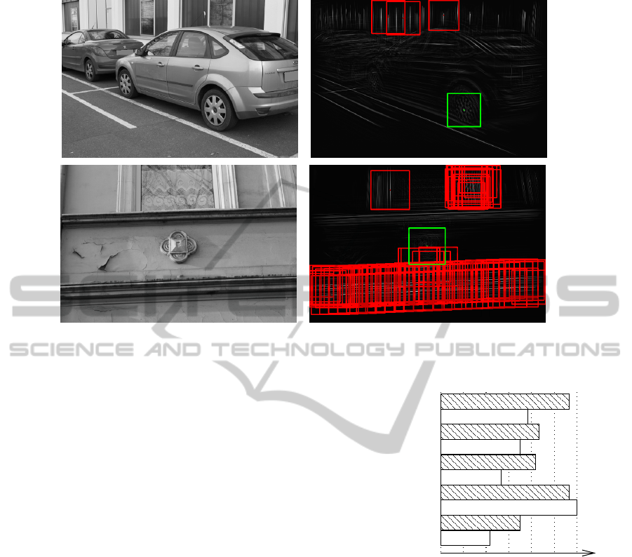
Figure 5: Some input images (left) and the corresponding symmetry transforms and detected symmetry points highlighted in

green (right). The red points are local maxima with a higher symmetry score that have been rejected due to a too high “edge

directedness”.

the dominant rotational symmetry. In the case of our

method, we have sorted out the axial symmetries with

the following algorithm:

1. Find all local maxima in the symmetry transform

and sort them by their score value in descending

order.

2. Find the highest score value in this list that has an

“edge directedness” less than 0.27, which is an in-

dicator for a rotational symmetry instead of an ax-

ial symmetry, according to the results of Sec. 4.1.

Fig. 5 shows for sample images from our test set both

the resulting highest score and the higher scores that

have been sorted out by the second criterion.

Results on the CVPR 2011 Data Set. The CVPR

2011 data set was used at the workshop on symmetry

detection at CVPR 2011 for comparing two yet un-

published algorithms by Kim & Lee & Chee and by

Kondra & Petrosino with the algorithm by Loy & Ek-

lundh (Loy and Eklundh, 2006) . It consists of 42 im-

ages (including 4 doublets) of a size about 200 × 150

that had been harvested on the Internet; it includes

ground truth data of the symmetry centers and the

axes length of the elliptic symmetry regions.

In the experiments reported in (Rauschert et al.,

2011), the algorithms returned more than one symme-

try point per image and Rauschert et al. reported both

a recall and a precision value. As we only take into ac-

count the highest symmetry count, we can only mea-

0.10 0.2 0.3 0.4 0.60.5

Kondra Petrosino*

Kim, Lee, Chee*

Loy, Eklundh*

Loy, Eklundh

Reisfeld 90 (log)

Reisfeld 90

Reisfeld 95 (log)

Reisfeld 95

Our method (log)

Our method

Figure 6: Recognition rates of the tested algorithms on the

CVPR 2011 data set. Values with an asterisk are the preci-

sion values reported in (Rauschert et al., 2011).

sure the recognition rate as a precision value, i.e. the

number of returned symmetry points that actually cor-

respond to a ground truth symmetry. We have consid-

ered a symmetry to be found when the detected sym-

metry point had a distance less than 5 pixels from a

ground truth symmetry center.

The measured values for our algorithm and the al-

gorithm by Reisfeld et al. together with the results

reported in (Rauschert et al., 2011) can be seen in

Fig. 6. As our recognition rate is computed slightly

different from the precision value by Rauschert et al.,

we have given both values for the algorithm by Loy

& Eklundh, which shows that both rates are compara-

ble observables. The results show that our method is

comparable to the best method from the CVPR 2011

VISAPP2013-InternationalConferenceonComputerVisionTheoryandApplications

582

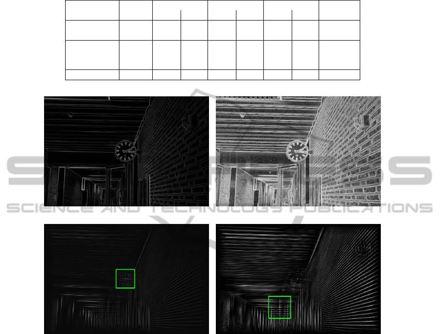
Table 1: Symmetry recognition rates on our test set for the different algorithms on different image categories (“Detail” etc.).

“grad” means that the gradient image has been used, while “log” means that the gradients have been transformed according

to Eq. (3).

Our method Reisfeld 95 Reisfeld 90 Loy &

Count grad log grad log grad log Eklundh

Detail 83 0.60 0.53 0.33 0.22 0.41 0.40 0.37

Context 76 0.33 0.39 0.18 0.20 0.37 0.36 0.37

Front 43 0.70 0.63 0.42 0.30 0.53 0.49 0.70

Light skew 57 0.58 0.53 0.25 0.14 0.47 0.40 0.39

Strong skew 59 0.20 0.29 0.15 0.20 0.20 0.27 0.12

Total 159 0.47 0.47 0.26 0.21 0.39 0.38 0.37

(a) Gradient absolute values. (b) Gradient absolute values after applying Eq. (3).

Figure 7: Effect of the logarithmic gradient transformation according to Eq. (3) on a sample image from our own data set.

The detected symmetries by our algorithm are highlighted in green.

workshop. A closer look at the individual images

showed that our algorithm performed best on the 15

images with C

∞

symmetries (0.73 versus 0.60 by Loy

& Eklundh), which is easily understandable as the

discrete C

symmetries also include some odd n, for

which our algorithm is less suited. Due to the small

number of images, this difference in the recognition

rate is however of limited signiﬁcance. It is interest-

ing to observe that a gradient transformation accord-

ing to Eq. (3) did not improve the symmetry detection,

but deteriorated the total recognition rate slightly. A

possible explanation can be that this transformation

ampliﬁes background and noise edges, as can be seen

in Fig. 7.

Results on our Own Data Set. To test the robust-

ness of the algorithms with respect to skew and back-

ground noise on a larger data base, we have addition-

ally run the algorithms on our own data set. Due to

the larger image size, we have here considered a sym-

metry point as correctly detected when the resulting

point had a distance less than 10 pixels from a ground

truth symmetry point.

The recognition rates of correctly detected sym-

metry points in Tbl. 1 show, somewhat surprisingly,

that the later 1995 method by Reisfeld et al. per-

formed poorer than their 1990 method, a difference

that was even signiﬁcant for a signiﬁcance level of 5%

according to McNemar’s test (Diettrich, 1998). Our

new method was better than the 1990 method by Re-

isfeld. Again, the gradient transformation according

to Eq. (3) deteriorated the symmetry detection. As the

deteriorating effect can be observed on both different

tested data sets, we conclude that the logarithmic nor-

DetectionofSymmetryPointsinImages

583

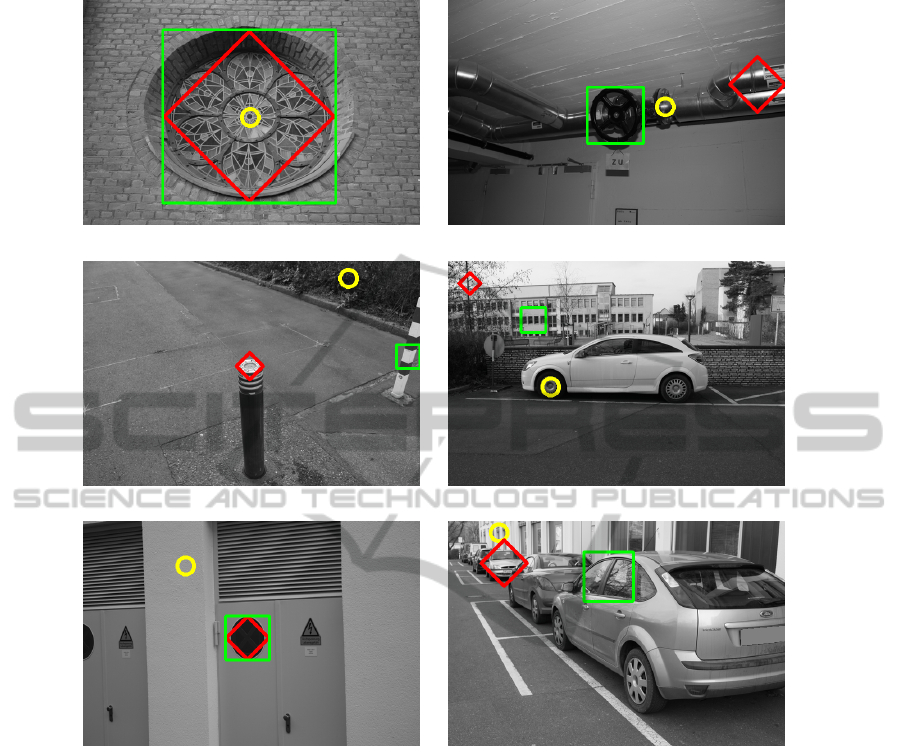
(a) (b)

(e) (f)

Figure 8: Some input images and the detected dominant rotational symmetry by our algorithm (green squares), and the

algorithms by Reisfeld et al. 1990 (red diamonds) and Loy & Eklundh (yellow circles).

malization of the gradient cannot be recommended for

symmetry detection.

Of all tested algorithms, the new method per-

formed on average even better than the algorithm by

Loy & Eklundh, which had shown the best perfor-

mance in the studies (Park et al., 2008) and (Rauschert

et al., 2011). As the varying results for the cate-

gories front/skewed show, the recognition rates of all

algorithms are lower for skewed rotation symmetries.

The algorithm by Loy & Eklundh is most suscep-

tible to distortion due to perspective: for unskewed

symmetries it shows the same performance as our al-

gorithm, but with skew the recognition rates become

even lower than those of the algorithm by Reisfeld et

al.. This is presumably due to the fact that a rotational

symmetry no longer holds in this case, but approxi-

mately becomes a C

mirror symmetry, which is still

detected by our method. Under stronger skew, this

approximation no longer holds and our method also

fails to detect most symmetries.

Fig. 8 shows exemplary results of all three al-

gorithms on images from our data set. There were

a number of images on which all three algorithms

worked well (like 8(a)), as well as images on which

all algorithms failed (e.g. due to a too strong skew

like in 8(f)). Neither algorithm was however consis-

tently better than a different algorithm on all images:

for each algorithm, there were images on which it was

the only one that detected a symmetry (see 8(b)-8(d)).

5 CONCLUSIONS

The new symmetry transform proposed in this paper

VISAPP2013-InternationalConferenceonComputerVisionTheoryandApplications

584

is very easy to implement and has shown a symmetry

detection rate that was both better than the algorithm

by Loy & Eklundh and than the symmetry transform

by Reisfeld et al. Even though the qualitative runtime

complexity of O(nr

) is similar to the latter algorithm,

with n the number of image pixels and r the maximum

radius, the absolute runtime of the new method is

lower because the symmetry score computation only

involves scalar products. While the method primarily

computes a point reﬂection symmetry (C

symmetry)

score, these can be discriminated into axial and rota-

tion symmetries with a criterion for the “edge direct-

edness” in the symmetry transform around the sym-

metry point.

For the method by Reisfeld et al., our experiments

have shown interesting results: ﬁrst that the rotational

symmetry score RS proposed in their later paper (Re-

isfeld et al., 1995) performed worse than the score

CS from their earlier paper (Reisfeld et al., 1990).

Moreover, the logarithmic transformation of the gra-

dients did not have the positive effect that Reisfeld

at al. have conjectured, which leads to the question

whether other transformations might be helpful. To-

gether with the question of an optimal choice for the

parameter σ, these are interesting points that require

more detailed investigations.

For the new symmetry transform, there are also

a number of interesting open questions for future re-

search. One is the evaluation and optimization of the

automatic radius detection. Others are the extension

of the radius detection to rectangular symmetric re-

gions, or the effect of other gradient transformations.

Another important question for every kind of symme-

try transform is what absolute criteria actually deter-

mine a symmetry point, a problem that we have cir-

cumvented in the present study by using the relative

criterion of the highest score in the image.

It should be noted that the application of the new

symmetry transform is not necessarily restricted to

symmetry detection. It may also be a useful starting

point for feature extraction from images.

REFERENCES

Diettrich, T. (1998). Approximate statistical tests for com-

paring supervised classiﬁcation learning algorithms.

Neural Computation, 10:1895–1923.

Gonzalez, R. and Woods, R. (2002). Digital Image Process-

ing. Prentice-Hall, New Jersey, 2nd edition.

Kanade, T. (1981). Recovery of the three-dimensional

shape of an object from a single view. Artiﬁcial In-

tellgence, 17:409–460.

Kuehnle, A. (1991). Symmetry-based recognition of vehi-

cle rears. Pattern recognition Letters, 12:249–258.

Lee, S. and Liu, Y. (2010). Skewed rotation symmetry

group detection. IEEE Transactions on Pattern Anal-

ysis and Machine Intelligence, 32(2):1659–1671.

Liu, Y., Hel-Or, H., Kaplan, C., and Gool, L. V. (2009).

Computational symmetry in computer vision and

computer graphics. Foundations and Trends in Com-

puter Graphics and Vision, 5:1–195.

Lowe, D. (2004). Distinctive image features from scale-

invariant keypoints. International Journal of Com-

puter Vision, 10(2):91–110.

Loy, G. and Eklundh, J. (2006). Detecting symmetry and

symmetric constellations of features. In European

Conference on Computer Vision (ECCV), pages 508–

521.

Loy, G. and Zelinsky, A. (2003). Fast radial symmetry for

detecting points of interest. IEEE Transactions on Pat-

tern Analysis and Machine Intelligence, 25(8):959–

973.

Park, M., Lee, S., Chen, P., Kashyap, S., Butt, A., and Liu,

Y. (2008). Performance evaluation of state-of-the-art

discrete symmetry detection algorithms. In IEEE Con-

ference on Computer Vision and Pattern Recognition

(CVPR), pages 1–8.

Rauschert, I., Brockelhurst, K., Liu, J., Kashyap, S., and

Liu, Y. (2011). Workshop on symmetry detection from

real world images - a summary. In IEEE Conference

on Computer Vision and Pattern Recognition (CVPR).

Reisfeld, D., Wolfson, H., and Yeshururn, Y. (1990). Detec-

tion of interest points using symmetry. In 3rd Interna-

tional Conference on Computer Vision, pages 62–65.

Reisfeld, D., Wolfson, H., and Yeshururn, Y. (1995).

Context-free attentual operators: The generalized

symmetry transform. International Journal of Com-

puter Vision, 14:119–130.

Tao, C., Shanxua, D., Fangrui, L., and Ting, R. (2009). Face

and facial feature localization based on color segmen-

tation and symmetry transform. In International Con-

ference on Multimedia Information Networking and

Security (MINES), pages 185–189.

DetectionofSymmetryPointsinImages

585